Chapter 1
Mathematical Preliminaries

In this introductory chapter, we will get familiar with vectors, tensors and various mathematical operations involving them. The concepts covered here will be used throughout the book. Hence, they are of paramount importance.

1.1 A vector and its representation: NPTEL link

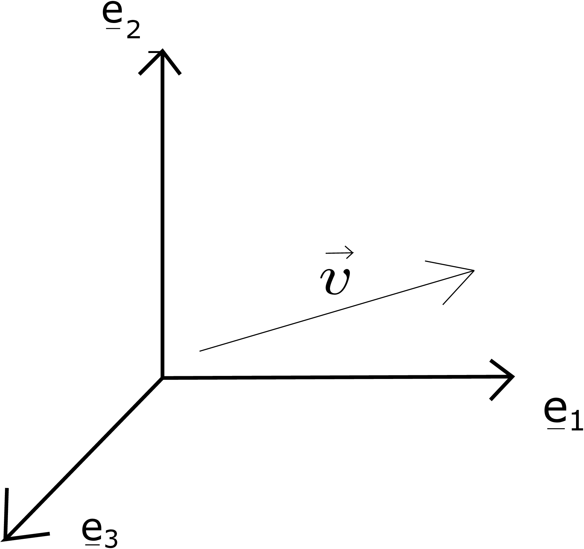
In layman’s term, a vector has both magnitude and direction. It is denoted by an arrow as shown in Figure 1.1. The length of the arrow signifies the vector’s magnitude while the arrow’s orientation signifies the vector’s direction.^∗ We have also shown a Cartesian coordinate system there whose basis vectors are (\(\underline {e}_1, \underline {e}_2\), \(\underline {e}_3\)). The component of a vector \(\overrightarrow {v}\) along the basis vector \(\underline {e}_i\) is given by \begin {equation} v_i = \overrightarrow {v}\cdot \underline {e}_i. \end {equation} Geometrically, this implies projection of the vector on to the basis vector \(\underline {e}_i\). The three components of a vector can be written together in a column form which we denote by the symbol \(\begin {bmatrix}\overrightarrow {v}\end {bmatrix}_{(\underline {e}_1, \underline {e}_2, \underline {e}_3)}\) and write \begin {equation} \begin {bmatrix}\overrightarrow {v}\end {bmatrix}_{(\underline {e}_1, \underline {e}_2, \underline {e}_3)}=\begin {bmatrix}v_1\\v_2\\v_3\end {bmatrix}. \end {equation} The subscript in \(\begin {bmatrix}\overrightarrow {v}\end {bmatrix}_{(\underline {e}_1, \underline {e}_2, \underline {e}_3)}\) signifies the coordinate system relative to which the vector components have been obtained. At this point, one should note that \(\begin {bmatrix}\overrightarrow {v}\end {bmatrix}_{(\underline {e}_1, \underline {e}_2, \underline {e}_3)}\) and \(\overrightarrow {v}\) are not the same: the former is the representation of the latter in the specified coordinate system. More importantly, a vector is independent of the coordinate system but its representation changes from one coordinate system to the other. To elaborate this point, think of a unit vector \(\overrightarrow {v}\) lying in space and being viewed from two different coordinate systems having basis vectors (\(\underline {e}_1,\underline {e}_2\), \(\underline {e}_3\)) and (\(\hat {\underline {e}}_1,\hat {\underline {e}}_2\), \(\hat {\underline {e}}_3\)) respectively - see Figure 1.2. The dashed coordinate system there can be obtained by rotating the black coordinate system by 45\(^{\circ }\) about \(\underline {e}_3\) axis.

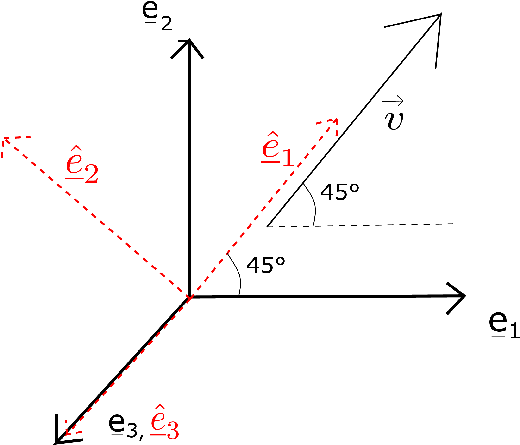
The vector \(\overrightarrow {v}\) itself lies in \(\underline {e}_1\) - \(\underline {e}_2\) plane and makes an angle of 45\(^{\circ }\) from \(\underline {e}_1\) axis. This also implies that \(\overrightarrow {v}\) is directed along \(\hat {\underline {e}}_1\), i.e., the first basis vector of the dashed coordinate system. The representation of \(\overrightarrow {v}\) in the two coordinate systems will thus be \begin {equation} \begin {bmatrix} \overrightarrow {v} \end {bmatrix}_{(\underline {e}_1,\underline {e}_2,\underline {e}_3)} = \begin {bmatrix} \frac {1}{\sqrt {2}}\\ \frac {1}{\sqrt {2}}\\0 \end {bmatrix} ,\quad \begin {bmatrix} \overrightarrow {v} \end {bmatrix}_{(\underline {\hat {e}}_1,\underline {\hat {e}}_2,\underline {\hat {e}}_3)} = \begin {bmatrix} 1\\0\\0 \end {bmatrix}. \end {equation} Thus, the representation (column form) of a vector varies from one coordinate system to the other but the vector itself is still directed in the same way in space and hence is independent of the coordinate system. It is also useful to note the below form for a vector:

From now on, we will denote a vector \(\overrightarrow {v}\) by \(\underline {v}\), i.e, instead of the overhead arrow, we will use an underbar.

1.2 Dot-product, Cross-product and Tensor-product of two vectors: NPTEL link

Let us now talk about three ways in which two vectors can be operated together. We begin first with dot product. The dot product of two vectors yields a scalar quantity and hence it is also called the scalar product. It is defined as follows:

Basically, the dot product of two vectors is obtained by summing the product of the corresponding components of those two vectors. From this definition, it appears that the dot product will be different in different coordinate systems since it involves the components of two vectors. However, as per the second formula above which is geometric in nature, it also equals the product of the magnitude of the two vectors multiplied by cosine of the angle between them. The second definition implies that the dot product of two vectors is independent of the coordinate system since neither the magnitude of a vector nor does the angle between two vectors change upon change of coordinate system.

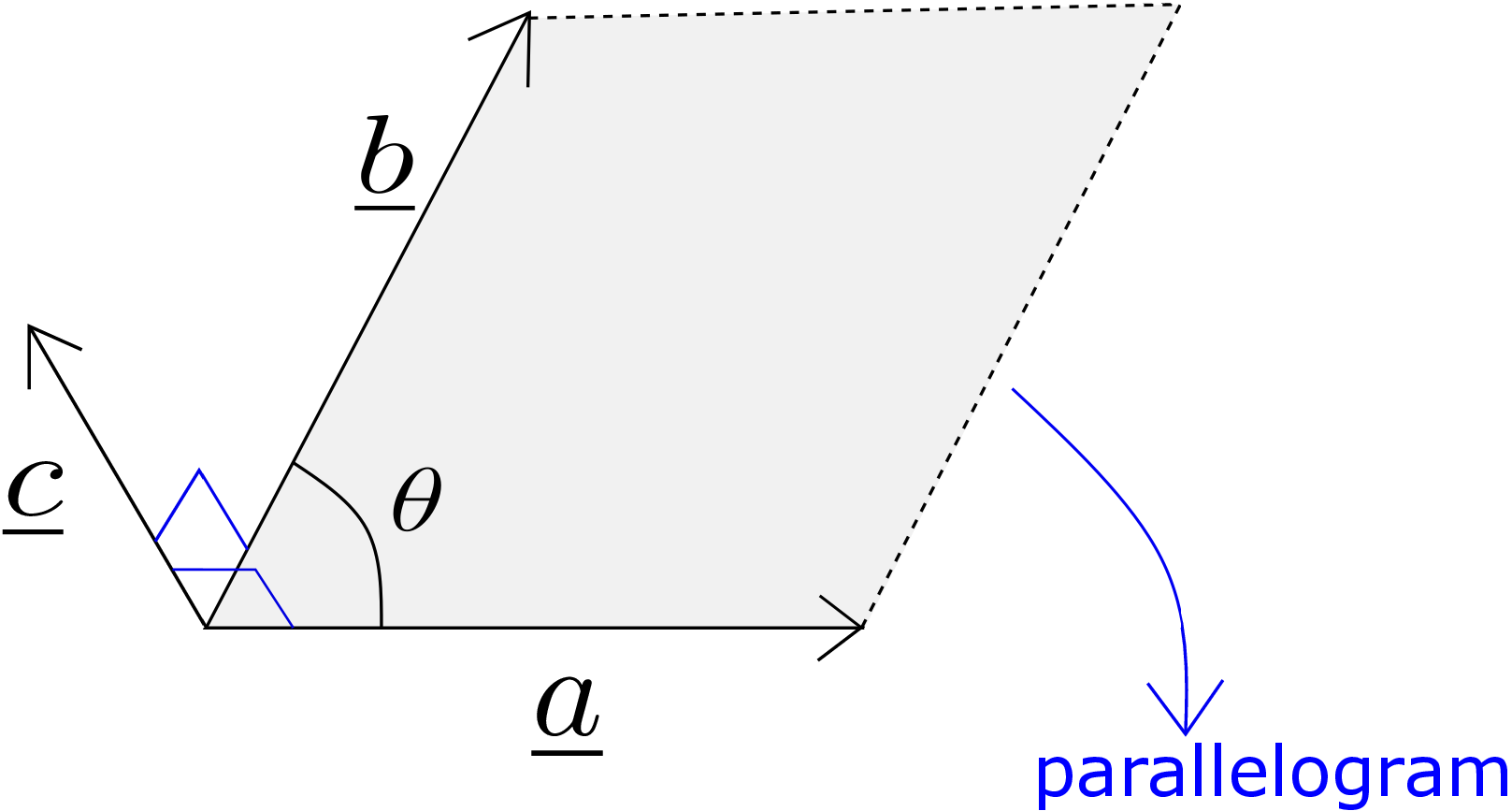
The cross product of two vectors yields a vector due to which it is also called the vector product. Like dot product, it is also independent of the coordinate system. Geometrically, it is defined as follows: \begin {equation} \underline {a}\times \underline {b}=\vert \vert \underline {a}\vert \vert ~\vert \vert \underline {b}\vert \vert ~ sin(\theta )~\underline {c}. \end {equation} Here \(\underline {c}\) is a unit vector perpendicular to the plane formed by \(\underline {a}\) and \(\underline {b}\). Its direction is given by the right hand thumb rule: when we curl our fingers from \(\underline {a}\) towards \(\underline {b}\), the thumb points towards \(\underline {c}\). The cross-product also equals the area vector of a parallelogram whose sides are formed by \(\underline {a}\) and \(\underline {b}\) (see Figure 1.3 for a graphical illustration). In a coordinate system, say (\(\underline {e}_1,\underline {e}_2\), \(\underline {e}_3\)), the cross product can be written as follows: \begin {equation} \label {1_cross_product} \begin {bmatrix}\underline {a}\times \underline {b}\end {bmatrix}_{(\underline {e}_1,\underline {e}_2, \underline {e}_3)}=\begin {bmatrix} \underline {a} \end {bmatrix}_{(\underline {e}_1,\underline {e}_2, \underline {e}_3)}\times \begin {bmatrix} \underline {b} \end {bmatrix}_{(\underline {e}_1,\underline {e}_2, \underline {e}_3)}= \begin {bmatrix} (a_2b_3-a_3b_2)\\(a_3b_1-a_1b_3)\\(a_1b_2-a_2b_1) \end {bmatrix}= \begin {bmatrix} 0 & -a_3 & a_2\\a_3 & 0 & -a_1\\-a_2 & a_1 & 0 \end {bmatrix} \begin {bmatrix} b_1\\b_2\\b_3 \end {bmatrix}. \end {equation} Thus, the cross product of two vectors can also be realized as the product of a skew symmetric matrix (a matrix whose diagonal elements are 0 and off-diagonal elements are negative of each other) times the column of the second vector. The components of the skew-symmetric matrix are formed by the components of the first vector \(\underline {a}\). In order to easily remember how to form the skew-symmetric matrix from the components of \(\underline {a}\), one can think of the following trick: to get the component in the \(i^{th}\) row and \(j^{th}\) column, the component of \(\underline {a}\) that will be used will be the third index (other than i and j). For example, for \(1^{st}\) row and \(2^{nd}\) column of the matrix, \(3^{rd}\) component \(a_3\) will be used. One then just has to remember where to place the negative signs. We also say \begin {equation} \begin {bmatrix} \underline {a} \end {bmatrix} = \begin {bmatrix} a_1\\a_2\\a_3 \end {bmatrix} =axial \begin {bmatrix} 0 & -a_3 & a_2\\a_3 & 0 & -a_1\\-a_2 & a_1 & 0 \end {bmatrix}. \end {equation} Basically, whenever we have a skew symmetric matrix, we can form a column from the three independent entries of that matrix and call the resultant column the axial/axial vector of that skew symmetric matrix.

Let us now talk of tensor product. This is a different kind of product which we may not have heard of yet. Through this product, we will also introduce a general notion of tensors. The tensor product of two vectors yields what is called a second order tensor which we write as follows: \begin {equation} \underline {a}\otimes \underline {b}= \underline {\underline {C}}. \end {equation} Here \(\underline {\underline {C}}\) (with two underbars) denotes a second order tensor. The tensor product is represented as follows in a coordinate system: \begin {equation} \label {1_tensor_representation} \begin {bmatrix} \underline {\underline {C}} \end {bmatrix}_{(\underline {e}_1,\underline {e}_2, \underline {e}_3)}=\begin {bmatrix}\underline {a}\otimes \underline {b}\end {bmatrix}_{(\underline {e}_1,\underline {e}_2, \underline {e}_3)}= \begin {bmatrix} \underline {a} \end {bmatrix}_{3\times 1} ~\left (\begin {bmatrix} \underline {b} \end {bmatrix}_{3\times 1}\right )^T. \end {equation} Notice that the tensor product implies that the second vector is transposed. This is in contrast with the dot product where the first vector is transposed. The above definition implies that the representation of this second order tensor C is a matrix whose individual components are given by \begin {equation} C_{i j}=a_i ~b_j. \end {equation}

1.3 Second order tensors and their representation: NPTEL link

The tensor product could also be written as follows:

Notice that we can move scalars anywhere in an expression, e.g., we moved \(b_j\) from right to left of the tensor product symbol and further to the left of vector \(\underline {e}_i\). We cannot do the same with vectors, e.g., we cannot change the order of appearance of the two vectors. Upon contrasting the above form with the expansion of a vector in equation \eqref{1_vector_expansion}, we make a note that, just like a general vector is expressed as a linear combination of three basis vectors, a second order tensor can be expressed as a linear combination of nine basis tensors. Each of the basis tensors (\(\underline {e}_i\otimes \underline {e}_j\)) here are themselves tensors. A general second order tensor can be written as follows: \begin {equation} \label {1_general_tensor} \underline {\underline {C}}=\sum _i\sum _j C_{ij}~ \underline {e}_i\otimes \underline {e}_j. \end {equation} The nine coefficients in \(C_{ij}\) are, in general, independent of each other. The coefficient \(C_{ij}\) can be thought of as the component of the tensor \(C\) along the basis tensor \(\underline {e}_i\otimes \underline {e}_j\). Using \eqref{1_tensor_representation}, we can also write the following for one of the basis tensors: \begin {equation} \label {1_basis_tensor} \begin {bmatrix}\underline {e}_1\otimes \underline {e}_2\end {bmatrix}_{(\underline {e}_1,\underline {e}_2, \underline {e}_3)}= \begin {bmatrix} 1\\0\\0 \end {bmatrix} \begin {bmatrix} 0 & 1 & 0 \end {bmatrix}= \begin {bmatrix} 0 & 1 & 0\\0 & 0 & 0\\0 & 0 & 0 \end {bmatrix}. \end {equation} Thus, just like basis vectors \(\underline {e}_i\) have column form, each of the basis tensors has a matrix form. Using \eqref{1_general_tensor} and \eqref{1_basis_tensor}, it is easy to see that the coefficient \(C_{ij}\) in \eqref{1_general_tensor} also forms the \(i^{th}\) row and \(j^{th}\) column of the matrix representation of \(\underline {\underline {C}}\) in (\(\underline {e}_1,\underline {e}_2, \underline {e}_3\)) coordinate system, i.e, \(\begin {bmatrix}\underline {\underline {C}}\end {bmatrix}_{(\underline {e}_1,\underline {e}_2, \underline {e}_3)}\). Just like vectors, the matrix form of a tensor changes from one coordinate system to the other but the tensor itself does not change, e.g., \begin {equation} \underline {\underline {C}}=\sum _i\sum _j C_{ij}~ \underline {e}_i\otimes \underline {e}_j= \sum _i\sum _j \hat C_{ij} ~\underline {\hat e}_i\otimes \underline {\hat e}_j. \end {equation} \begin {equation*} \qquad \downarrow \text {(matrix form)}\downarrow \end {equation*} \begin {equation*} \quad ~~\begin {bmatrix} C_{ij} \end {bmatrix}\qquad \qquad \quad \begin {bmatrix} \hat C_{ij} \end {bmatrix} \end {equation*} Thus, we get different matrices in different coordinate system but the tensor itself is still the same. As a final remark, tensors can be of any order which are all independent of the coordinate system but their representations change from one coordinate system to the other. For example, all scalars are zeroth order tensors whereas all vectors are first order tensors. We can also have third and fourth (even higher) order tensors. A common question often comes to our mind. There are several examples of vectors in real life (velocity, force etc.). Do tensors exist in reality or are they abstract quantities? We will have a clearer answer to this question as we progress through the book. We also have the concept of transpose of a tensor. For a second order tensor \(\underline {a}\otimes \underline {b}\), its transpose is defined to be \(\underline {b}\otimes \underline {a}\). For a general second order tensor of the form \begin {equation} \label {1_definition1} \underline {\underline {A}} = \sum _{i} \sum _{j} A_{ij} \; \underline {e}_{i} \otimes \underline {e}_{j}, \end {equation} we can write its transpose to be \begin {equation} \underline {\underline {A}}^T = \sum _i \sum _{j} A_{ij} \; \underline {e}_{j} \otimes \underline {e}_{i}. \end {equation} Basically, the order of two vectors in tensor product operation is flipped. Upon further renaming \(i \rightarrow j\) and \(j \rightarrow i\), we get \begin {equation} \label {1_definition2} \underline {\underline {A}}^T = \sum _{j} \sum _{i} A_{ji} \; \underline {e}_{i} \otimes \underline {e}_{j}. \end {equation} From definitions \eqref{1_definition1} and \eqref{1_definition2}, one can then realize that the matrix form of transpose of \(\underline {\underline {A}}\) is equal to the transpose of the matrix form of \(\underline {\underline {A}}\), i.e., \[ [\underline {\underline {A}}^T] = [\underline {\underline {A}}]^T. \]

1.4 Multiplying a second order tensor with a vector: dot product and tensor product: NPTEL link

Just like there are several ways in which two vectors can be multiplied (scalar product, vector product, tensor product), the same can be said about multiplication of a second order tensor with a vector.

We start with the dot product of a tensor with a vector. It is also called single contraction and is defined as follows:

Often, the dot symbol is suppressed when we mean this single contraction. To proceed further, the second vector from the 2nd order tensor is dotted with the first order tensor, i.e.,

Here \(\delta _{jk}\) is called the Kronecker delta function and is defined as follows:

Now consider the summation over \(k\) in \eqref{1_tensor_vector}. Due to the Kronecker delta function present there, only the term having \(k=j\) will contribute to the summation and others will be zero. Thus, we can get rid of the summation over \(k\) and replace \(k\) by \(j\) at all places, i.e., \begin {equation} \underline {a}=\underline {\underline {C}}\cdot \underline {b}=\sum _i\left (\sum _j C_{ij} b_j\right )~\underline {e}_i. \end {equation} As any general vector can be written as \(\underline {a}=\sum _i a_i~\underline {e}_i\), the term in the parentheses above turns out to be \(a_i\). Thus, when we dot product/single contract a second order tensor with a vector, we get a vector whose components are given by

\begin {equation*} \qquad \qquad \searrow \end {equation*} \begin {equation*} \qquad \qquad \qquad i^{th}\hspace {2mm} row\hspace {2mm} of \begin {bmatrix} \underline {\underline {C}} \end {bmatrix} \end {equation*} \begin {equation} \Rightarrow \begin {bmatrix} a_1\\a_2\\a_3 \end {bmatrix}= \begin {bmatrix} \underline {\underline {C}} \end {bmatrix} \begin {bmatrix} \underline {b} \end {bmatrix}.\label {1_matrix_times_vector} \end {equation} Thus, we simply multiply the matrix form of \(C\) with the column form of \(b\) in the usual way to get the column form of the resulting vector \(a\). At this point, let us recall the cross product definition in \eqref{1_cross_product} where we had written it as a skew symmetric matrix times a vector. On further noting the multiplication we just saw in \eqref{1_matrix_times_vector}, we immediately conclude that the cross product of two vectors can also be thought of as a second order tensor dotted with the second vector where the second order tensor corresponds to the first vector, i.e., \begin {equation} \underline {c}=\underline {a}\times \underline {b}= \underline {\underline {a}}\cdot \underline {b}. \end {equation} We also have tensor product of a second order tensor with a vector: the outcome is a third order tensor. It is defined as follows:

Extracting the coefficients in the matrix representation of a second order tensor

To get the coefficient, say \(C_{kl}\), of the matrix form of a tensor \(\underline {\underline {C}}\) in \((\underline {e}_1,\underline {e}_2,\underline {e}_3)\) coordinate system, we’ll verify that \begin {equation} \label {1_extracting_tensor_coefficient} C_{kl}=(\underline {\underline {C}}\cdot \underline {e}_l)\cdot \underline {e}_k. \end {equation} Let us write the above equation in \((\underline {e}_1,\underline {e}_2,\underline {e}_3)\) coordinate system for \(k=1,l=2\): \begin {equation*} (\underline {\underline {C}}\cdot \underline {e}_2)\cdot \underline {e}_1= \left ( \begin {bmatrix} C_{11} & C_{12} & C_{13}\\C_{21} & C_{22} & C_{23}\\C_{31} & C_{32} & C_{33} \end {bmatrix} \begin {bmatrix} 0\\1\\0 \end {bmatrix} \right )\cdot \begin {bmatrix} 1\\0\\0 \end {bmatrix}= \begin {bmatrix} C_{12}\\C_{22}\\C_{32} \end {bmatrix}\cdot \begin {bmatrix} 1\\0\\0 \end {bmatrix}=C_{12}. \end {equation*} This verifies equation \eqref{1_extracting_tensor_coefficient}. Stated differently, by using equation \eqref{1_extracting_tensor_coefficient}, we are able to extract the component of an arbitrary second order tensor \(\underline {\underline {C}}\) relative to the basis tensor \(\underline {e}_k\otimes \underline {e}_l\).

1.5 Multiplying two second order tensors: single-contraction, double-contraction and tensor product: NPTEL link

There are again various ways in which two second order tensors can be operated together. We begin with single contraction. The single contraction of two second order tensors yields another second order tensor. This single contraction is defined as follows:

Using Kronecker delta property, we then remove the summation over \(j\) and replace \(j\) with \(k\), i.e.,^†

This is the expression for C and a general second order tensor C can be written as \(\sum _i \sum _l C_{il}\hspace {1mm}\underline {e}_i \otimes \underline {e}_l\) (using equation \eqref{1_general_tensor}). Noting this in the above expression, we see that the expression within the bracket is \(C_{il}\), i.e.,

\begin {equation*} \quad \qquad \qquad \qquad \qquad \quad \searrow \qquad \quad \searrow \end {equation*} \begin {equation*} \hspace {6cm}i^{th}\hspace {2mm}row\hspace {2mm}of\hspace {2mm}\begin {bmatrix} \underline {\underline {a}} \end {bmatrix}, \hspace {2mm}l^{th}\hspace {2mm}column\hspace {2mm}of\hspace {2mm}\begin {bmatrix} \underline {\underline {b}} \end {bmatrix} \end {equation*} Writing this for all components together, we get \begin {equation} \begin {bmatrix} \underline {\underline {C}} \end {bmatrix}= \begin {bmatrix} \underline {\underline {a}} \end {bmatrix} \begin {bmatrix} \underline {\underline {b}} \end {bmatrix}. \end {equation} Thus, we see that when two second order tensors are single-contracted, their matrix forms multiply in the usual way: the matrix form of the resultant tensor is simply the multiplication of the matrix forms of individual tensors.

The double contraction of two second order tensors yields a scalar and is defined as follows:

By definition, the corresponding vectors on two sides of “double contraction” are dotted, i.e., \(\underline {e}_i\) with \(\underline {e}_k\) and \(\underline {e}_j\) with \(\underline {e}_l\). We thus obtain

Basically, the corresponding components of two tensors are multiplied and summed - this is very much like we do in dot product of two vectors.

We then talk of tensor product of two second order tensors. It yields a fourth order tensor as follows:

1.6 Calculus of tensors: divergence and gradient

The divergence of a tensor is defined as follows:

For example, for a first order tensor: \begin {align*} \begin {split} \ve {\nabla }\cdot \ve {v} = \msum {i} \dfrac {\partial }{\partial x_i}\brc {\ve {v}}\cdot \ve {e}_i=\msum {i}\dfrac {\partial }{\partial x_i}\brc {\msum {j} v_j \ve {e}_j}\cdot \ve {e}_i=\msum {i}\msum {j} \dfrac {\partial v_j}{\partial {x}_i}\delta _{ij}=\msum {i}\dfrac {\partial v_i}{\partial x_i}. \end {split} \end {align*}

The gradient of a tensor is defined as follows:

Notice its difference with the formula for the divergence of a tensor. The gradient of a vector \(\underline {f}\), e.g., is

It is a second order tensor whose matrix form is simply formed by the coefficient \(\frac {\partial f_i}{\partial X_j}\). Similarly, the gradient of a scalar quantity is defined as follows: \begin {equation} \underline {\nabla }\,{f}=\sum _i\frac {\partial {f}}{\partial X_i} \underline {e}_i. \end {equation} If we represent this vector in the coordinate system (\(\underline {e}_1\), \(\underline {e}_2\), \(\underline {e}_3\)), we get \begin {equation} \begin {bmatrix} \underline {\nabla }\,f \end {bmatrix}_{(\underline {e}_1,\underline {e}_2,\underline {e}_3)}= \begin {bmatrix} \dfrac {\partial f}{\partial X_1} & \dfrac {\partial f}{\partial X_2}& \dfrac {\partial f}{\partial X_3} \end {bmatrix}^T. \end {equation} This is the column from of gradient that we have seen in first year math course. Notice that divergence reduces the order of a tensor by 1 whereas gradient increases the order of a tensor by 1.

1.7 Rotation tensor: NPTEL link

As the name suggests, rotation tensors are related to physical rotation of objects. They can be used to rotate vectors as well as tensors. It should have the property such that after rotation, vectors and tensors do not change their magnitude but only direction. Let us consider two sets of orthonormal triads (see Figure 1.4: each set contains three vectors which are perpendicular to each other and also of unit magnitude). One can always transform a set of triad into another through a unique rotation or what we call a rotation tensor. Mathematically, we write \begin {equation} \label {1_Rotation_definition} \underline {\hat e}_i=\underline {\underline {R}}\hspace {1mm}\underline {e}_i~ \forall ~ i=1,2,3. \end {equation} The matrix form of this rotation tensor turns out to be an orthonormal (‘ortho’ means perpendicular and ‘normal’ means normalized) matrix. The tensor itself is called an orthonormal tensor. Orthonormal tensors and their matrix forms have the following properties: \begin {equation} \label {1_orthonormal} (a)~\underline {\underline {R}}\hspace {1mm}\underline {\underline {R}}^T=\underline {\underline {R}}^T\underline {\underline {R}}=\underline {\underline {I}}~(\text {an identity tensor}),\quad (b)~det(\underline {\underline {R}})=1. \end {equation}

This means that rows of \(\begin {bmatrix} \underline {\underline {R}} \end {bmatrix}\) are perpendicular to each other and are themselves normalized to be of unit magnitude, i.e., the rows are orthonormal with respect to each other. One can similarly prove that its columns are also orthonormal with respect to each other.

Let us consider an specific example and see what does a rotation matrix look like.

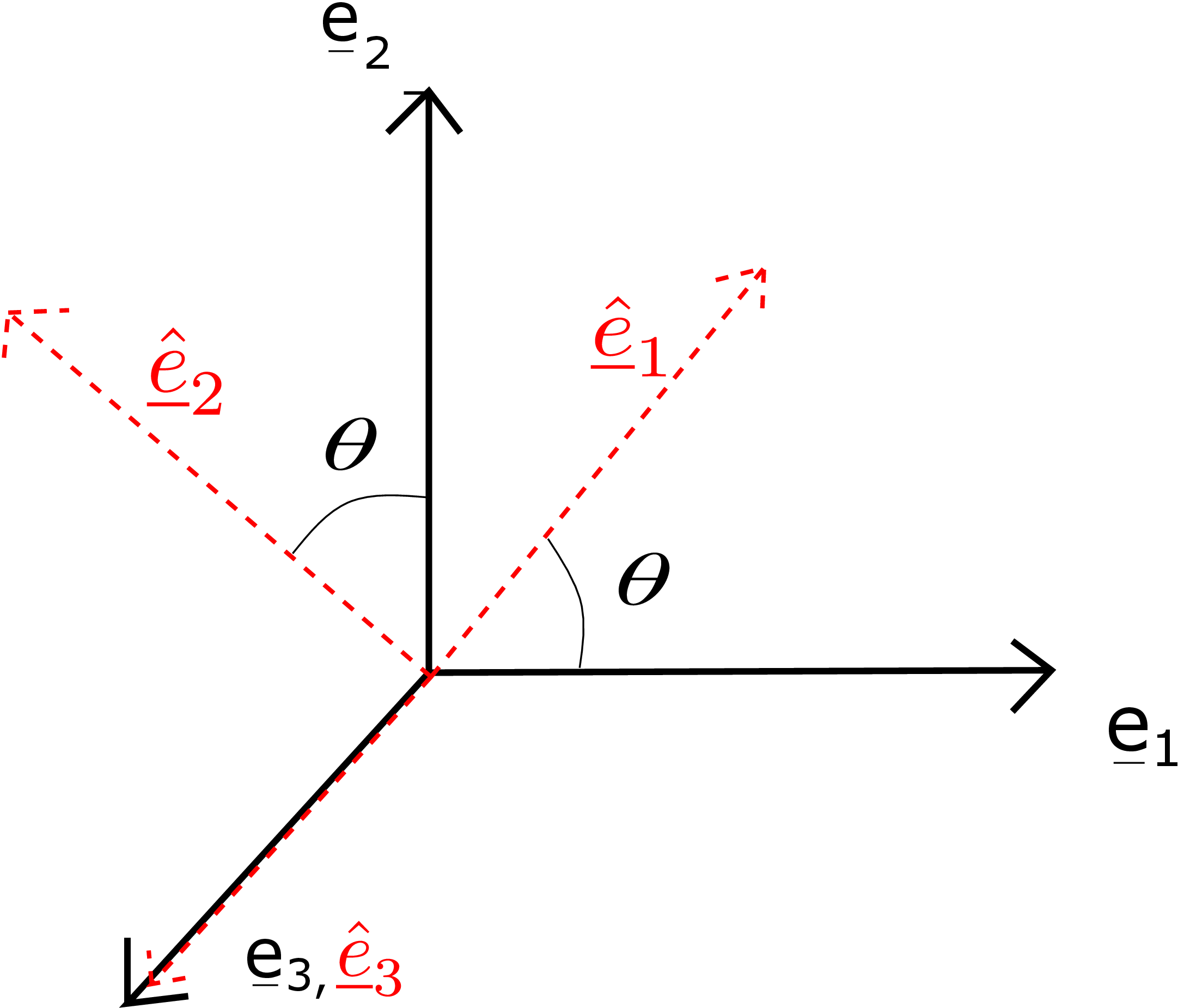
In Figure 1.5, we have (\(\underline {e}_1,\underline {e}_2,\underline {e}_3\)) coordinate system and it is rotated by \(\underline {\underline {R}}\) to get the new coordinate system (\(\underline {\hat e}_1,\underline {\hat e}_2,\underline {\hat e}_3\)). The rotation is such that \(\underline {\hat e}_3\) is same as \(\underline {e}_3\) and the other two basis vectors are rotated by \(\theta \). Let us determine the matrix form \(\begin {bmatrix} \underline {\underline {R}} \end {bmatrix}\) in (\(\underline {e}_1,\underline {e}_2,\underline {e}_3\)) coordinate system. We know from equation \eqref{1_extracting_tensor_coefficient} that

So, the \(j^{th}\) column of the rotation matrix is the column form of vector \(\underline {\hat e}_j\) expressed in (\(\underline {e}_1,\underline {e}_2,\underline {e}_3\)) coordinate system. For example, consider \(j\)=2: \begin {equation} R_{i2}=\underline {\hat e}_2\cdot \underline {e}_i. \end {equation} We can thus find these coefficients in terms of \(\theta \) using dot product definition, e.g., \begin {equation} \underline {\hat e}_2\cdot \underline {e}_1=-\text {sin}\theta , \quad \underline {\hat e}_2\cdot \underline {e}_2=\text {cos}\theta , \quad \underline {\hat e}_2\cdot \underline {e}_3=0. \end {equation} Working out all the components in this way, we get \begin {equation} \begin {bmatrix} \underline {\underline {R}} \end {bmatrix}_{(\underline {e}_1,\underline {e}_2,\underline {e}_3)}= \begin {bmatrix} cos\theta & -sin\theta & 0\\sin\theta & cos\theta & 0\\ 0 & 0 & 1 \end {bmatrix}. \end {equation} Note that the third column is \([0\hspace {1mm}0\hspace {1mm}1]^T\) as \(\underline {\hat e}_3\) is same as \(\underline {e}_3\). We emphasize that the above matrix form is the representation of rotation tensor \(\underline {\underline {R}}\) in \((\underline {e}_1,\underline {e}_2,\underline {e}_3)\) coordinate system. This matrix form will be different if we choose another coordinate system to represent the tensor.

As a side note, any rotation can be uniquely characterized by its axis of rotation (unit vector \(\underline {a}\)) and the angle of rotation \(\theta \). One can then use the following Rodrigue’s formula to obtain the rotation tensor in terms of these two information: \begin {equation} \underline {\underline {R}}(\underline {a},\theta )=\underline {\underline {I}} + sin(\theta )~\underline {\underline {a}} + (1-cos(\theta ))~\underline {\underline {a}}^2. \end {equation} Here \(\underline {\underline {a}}\) is a skew symmetric tensor whose axial vector is \(\underline {a}\).

1.8 Solved examples

Method 1 (using indical notation): \begin {align*} \va \cdot \brc {\mA \; \vb } &= \msum {i} a_{i} \ve {e}_{i} \cdot \sbk {\brc { \msum {j} \msum {k} A_{jk} \; \ve {e}_{j} \otimes \ve {e}_{k}} \cdot \msum {l} b_{l}\ve {e}_{l}}\\ &= \msum {i} a_{i} \ve {e}_{i} \cdot \msum {j} \msum {k} \msum {l} A_{jk} b_{l} \delta _{kl} \; \ve {e}_j\\ &= \msum {i} \msum {j} \msum {k} \msum {l} a_{i} A_{jk} b_{l} \delta _{kl} \delta _{ij}\\ &= \msum {j} \msum {l} a_{j} A_{jl} b_{l}\\ \brc {\mA ^{T} \va } \cdot \vb &= \sbk {\brc { \msum {j} \msum {k} A_{kj} \; \ve {e}_{j} \otimes \ve {e}_{k}} \cdot \msum {i} a_{i} \ve {e}_{i}} \cdot \msum {l} b_{l} \ve {e}_{l} \\ &= \msum {i} \msum {j} \msum {k} a_{i} A_{kj} \delta _{ki} \; \ve {e}_j \cdot \msum {l} b_{l} \ve {e}_{l} \\ &= \msum {i} \msum {j} \msum {k} \msum {l} a_{i} A_{kj} b_{l} \delta _{ki} \delta _{lj}\\ &= \msum {i} \msum {j} a_{i} A_{ij} b_{j} = \msum {j} \msum {l} a_{j} A_{jl} b_{j} \text { (due to renaming of dummy summation indices)} \end {align*}

Method 2 (using their matrix forms): \begin {align*} \begin {split} \va \cdot (\mA \; \vb ) & = \sva ^T \cmA \;\svb \\ & =\brc {\sva ^T \cmA \; \svb }^T \;\; (\because \text {transpose of a scalar remains the same})\\ & = \svb ^T \cmA ^T \sva \\ & = \svb ^T \brc {\cmA ^T \sva }\\ & = \svb \cdot \left [\mA ^T \va \right ] = \vb \cdot \brc {\mA ^T \va }. \end {split} \end {align*}

Solution: As per information provided: \(\mA \cdot \ve {e}_1 = \va \) \begin {align*} \begin {split} \text {or}~ \begin {bmatrix} A_{11}&A_{12}&A_{13}\\ A_{21}&A_{22}&A_{23}\\ A_{31}&A_{32}&A_{33} \end {bmatrix} \begin {bmatrix} 1\\0\\0 \end {bmatrix} &= \begin {bmatrix} a_{1}\\a_{2}\\a_{3} \end {bmatrix} \quad \text {(expressed in the sought coordinate system)}\\ \therefore \begin {bmatrix} A_{11}\\A_{21}\\A_{31} \end {bmatrix} &= \begin {bmatrix} a_{1}\\a_{2}\\a_{3} \end {bmatrix} \text { (1st column of $\cmA = \sva $)} \end {split} \end {align*}

One can similarly show that \begin {align*} \begin {bmatrix} A_{12}\\A_{22}\\A_{32} \end {bmatrix} = \begin {bmatrix} b_{1}\\b_{2}\\b_{3} \end {bmatrix} \text { (2nd column of $\cmA = \svb $)} \text { and } \begin {bmatrix} A_{13}\\A_{23}\\A_{33} \end {bmatrix} = \begin {bmatrix} c_{1}\\c_{2}\\c_{3} \end {bmatrix} \text { (3rd column of $\cmA = \svc $)}. \end {align*}

To see how the tensor form of \(\mA \) looks like, one can derive as follows: \begin {align*} \begin {split} \cmA &= \begin {bmatrix} A_{11}& 0 & 0\\ A_{21}& 0 & 0\\ A_{31}& 0 & 0 \end {bmatrix} + \begin {bmatrix} 0 & A_{12} & 0\\ 0 & A_{22} & 0\\ 0 & A_{32} & 0 \end {bmatrix} + \begin {bmatrix} 0 & 0 & A_{13}\\ 0 & 0 & A_{23}\\ 0 & 0 & A_{33} \end {bmatrix} \\ \text {or}~\cmA &= \sbk {\va } \sbk {\ve {e}_1}^T + \sbk {\vb } \sbk {\ve {e}_2}^T + \sbk {\ve {c}} \sbk {\ve {e}_3}^T \\ \text {or}~\mA &=\va \otimes \ve {e}_1+\vb \otimes \ve {e}_2+\ve {c}\otimes \ve {e}_3. \end {split} \end {align*}

(a) Let’s start with the matrix form of tensor expression \(\brc {\va \otimes \vb } \mC \) \begin {align*} \begin {split} \brc { \sva \; \svb ^T} \cmC &= \sva \brc {\svb ^T \cmC } \quad (\text {using associative rule of matrix multiplication})\\ &= \sva \brc {\cmC ^T \svb }^T = \va \otimes \brc {\mC ^T \vb } \end {split} \end {align*}

(b) Starting with the matrix form of tensor expression \(\matr {C} \brc {\va \otimes \vb } \) \begin {align*} \begin {split} \left [\mC \brc {\va \otimes \vb }\right ] = \cmC \brc { \sva \svb ^T} = \brc {\cmC \sva } \svb ^T = \brc {\mC \; \va } \otimes \vb . \end {split} \end {align*}

Solution: \begin {align*} \begin {split} \brc {\mA \;\ve {x}} \cdot \ve {x} &= \ve {x} \cdot \brc {\mA ^T \ve {x}}\\ &= - \ve {x} \cdot \brc {\mA \; \ve {x}}\\ &= - \brc {\mA \; \ve {x}} \cdot \ve {x} \text { (from commutative rule of dot-product of two vectors)}\\ &= 0 \text { (since only zero can be negative of itself!)} \end {split} \end {align*}

Disclaimer: The commutative rule (\(\va \cdot \vb = \vb \cdot \va \)) applies only for 1st-order tensors and does not extend to higher order tensors. For example, \(\mA \cdot \vb \ne \vb \cdot \mA \) or \(\mA \cdot \mC \ne \mC \cdot \mA \).

Solution: Recall that a tensor \(\mR \) remains invariant in different coordinate systems. However, its representation or its matrix form is different in different coordinate systems. Also, rotation tensors are orthonormal and satisfy the following property: \(\mR ^{-1} = \mR ^T\). Since \(\mR \) in the question maps \(\brc {\ve {e}_{1}, \ve {e}_{2}, \ve {e}_{3}}\rightarrow \brc {\hat {\ve {e}}_{1}, \hat {\ve {e}}_{2}, \hat {\ve {e}}_{3}}\), we can write \begin {align} \label {1_relation1} \begin {split} \hat {\ve {e}}_{i} = \mR \;\ve {e}_{i} \Rightarrow \mR ^{-1} \hat {\ve {e}}_{i} = \ve {e}_{i} ~\text {or}~ \mR ^{T} \hat {\ve {e}}_{i} = \ve {e}_{i}. \end {split} \end {align}

One can also write \begin {align*} \mR = \msum {i} \msum {j} \hat {R}_{ij} \; \hat {\ve {e}}_{i} \otimes \hat {\ve {e}}_{j} \end {align*}

where the components \(\hat {R}_{ij}\) can be obtained as follows: \begin {align*} \begin {split} \hat {R}_{ij} = \brc {\mR \; \hat {\ve {e}}_{j}} \cdot \hat {\ve {e}}_{i} = \hat {\ve {e}}_{j} \cdot \mR ^T \hat {\ve {e}}_{i} = \hat {\ve {e}}_{j} \cdot \ve {e}_{i}\quad \text {(using \eqref {1_relation1})} \end {split} \end {align*}

We had derived the same expression for \(R_{ij}\) earlier while discussing rotation tensors. This result is non-intuitive as we do not expect the representation of a tensor in two different coordinate systems to be the same in general. However, this case happens to be a special one since the given tensor also transforms the first coordinate system into other.

1.9 Objective questions to recall concepts

(1)

We can say the following about a tensor:

(a)

It is independent of the coordinate system

(b)

It changes from one coordinate system to other

(c)

Its representation changes from one coordinate system to another

(d)

None of the above

(2)

Which of the following statements is/are correct?

(a)

Scalars are zeroth order tensors

(b)

Tensors are independent of the coordinate system

(c)

Vectors are more general than tensors

(d)

One can add tensors of different orders

(3)

What is the product of a scalar with another vector?

(a)

It’s a vector

(b)

It’s a second order tensor

(c)

It’s a scalar

(d)

None of these

(4)

What is the product of a vector with another vector?

(a)

It’s a vector

(b)

It depends on whether we are doing dot product, cross-product or tensor product

(c)

Dot product gives a scalar quantity

(d)

None of these

(5)

Which of the following statements is/are correct concerning the cross product of two vectors?

(a)

Cross product of two vectors gives us a second order tensor.

(b)

Cross product of two vectors is the same as the product of a skew-symmetric tensor formed by the first vector times the second vector.

(c)

Cross product of two vectors is dependent on the coordinate system.

(d)

None of these

(6)

A second order tensor, in general, has

(a)

three independent coefficients

(b)

six independent coefficients

(c)

nine independent coefficients

(d)

none of these

(7)

What is the order of the tensor obtained from the dyadic product of two vectors?

(a)

Zeroth order

(b)

First order

(c)

Second order

(d)

None of these

(8)

Which of the following is/are incorrect concerning vectors?

(a)

The representation of a vector is different in different coordinate systems.

(b)

A vector is a second order tensor.

(c)

A vector is a first order tensor.

(d)

A vector remains the same irrespective of change in the coordinate system.

(9)

We can say the following about a rotation tensor.

(a)

It uniquely relates a set of three orthonormal vectors with another set of three orthonormal vectors

(b)

Any two columns of its matrix form are orthogonal to each other

(c)

The determinant of its matrix form equals -1

(d)

Its inverse equals its transpose

(10)

Which of the following is/are the property of a rotation tensor \(\underline {\underline {R}}\)?

(a)

\(\underline {\underline {R}}\underline {\underline {R}}^T=\underline {\underline {I}}\)

(b)

\(\det (\underline {\underline {R}})=1\)

(c)

\(\det (\underline {\underline {R}})= -1\)

(d)

\(\underline {\underline {R}}^T\underline {\underline {R}}=\underline {\underline {I}}\)

(11)

Which of the following is true for the tensor equation: \(\underline a\) =\(\underline {\underline {R}}\) \(\underline b\)?

(a)

It can be expressed/expanded only in \(\underline e_1\)-\(\underline e_2\)-\(\underline e_3\) coordinate system

(b)

It can be expressed/expanded in any coordinate system

(c)

It can be expressed/expanded only in that coordinate system in which we are working

(d)

None of these

1.10 Questions to practise

(1)

If \(\ve {a}\) and \(\ve {b}\) are two vectors, show that their dot product \(\ve {a} \cdot \ve {b}\) remain the same in different coordinate systems (say \(\brc {\ve {e}_{1}, \ve {e}_{2}, \ve {e}_{3}}\) and \(\brc {\hat {\ve {e}}_{1}, \hat {\ve {e}}_{2}, \hat {\ve {e}}_{3}}\)).

(2)

Prove that \( \sbk {\brc {\ve {u} \cdot \ve {a}} \brc {\matr {A}^T \ve {b}}} \cdot \ve {n} = \ve {a} \cdot \sbk {\brc {\ve {u} \otimes \matr {A} \ve {n}}} \ve {b} \).

(3)

If \(\matr {A}\) is a symmetric tensor and \(\matr {B}\) is an anti-symmetric tensor, then show that \[ \matr {A} : \matr {B} = 0. \]