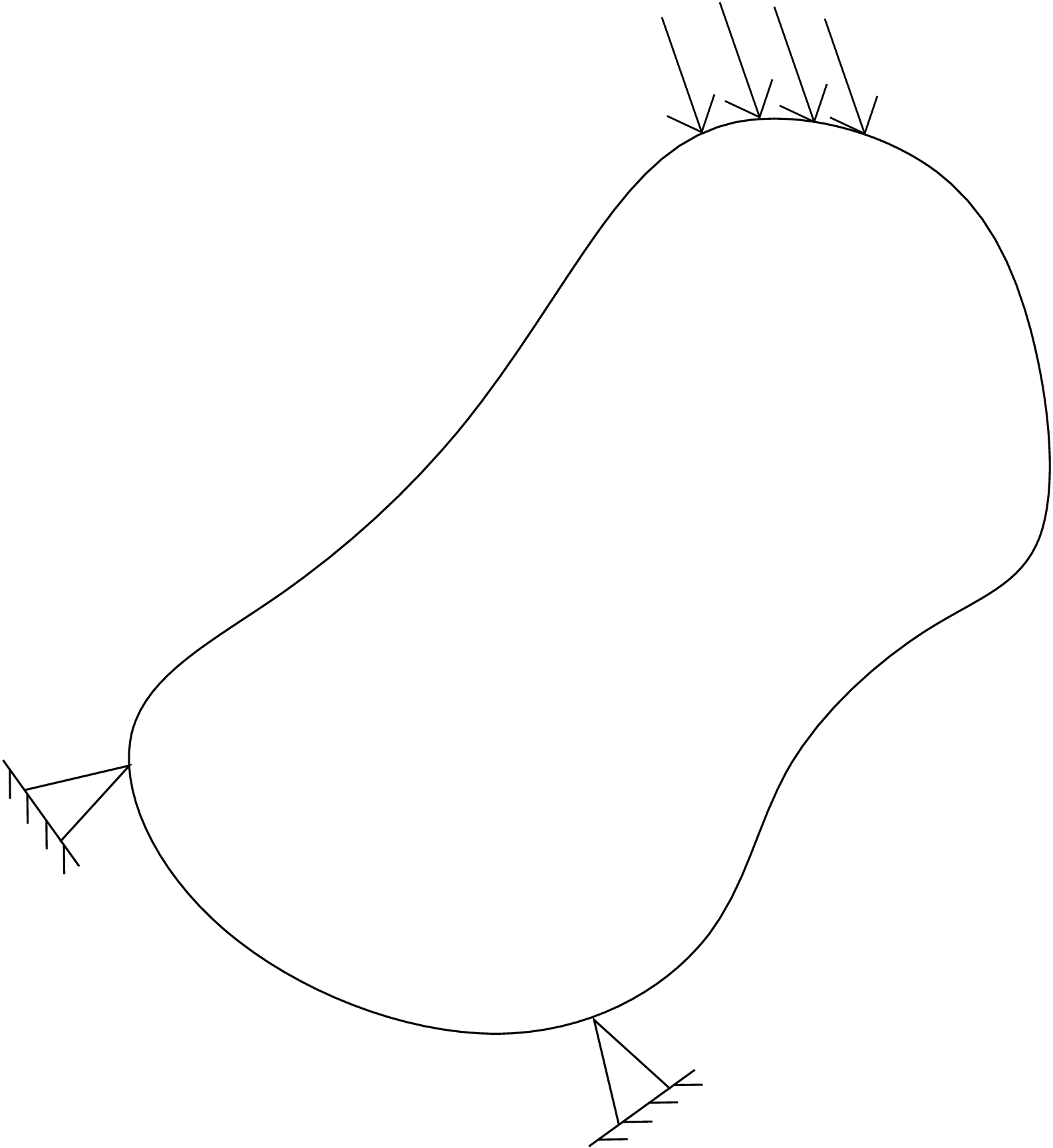
In this chapter, we will learn about various theories of failure and further apply them to solve few example problems. Let us begin with the motivation for this chapter. Think of an arbitrary body clamped at some points on its surface as shown in Figure 11.1.
It is further subjected to traction at some other parts of the surface. The body deforms due to the applied traction. As we increase the magnitude of applied traction, the body deforms more and more and at one point, the body will eventually fail. This failure can be in terms of the body suddenly getting deformed a lot (yielding or buckling) or due to crack developing in the body. The failure (e.g., due to crack) usually initiates at a point in the body and not at all points together. At each point in the body, a different state of stress and strain exists. If, at a point, some function of stress or strain components reaches a critical value, failure occurs. The different theories of failure have been developed on the basis of the specific form of the failure function in terms of stress/ strain components. For example, failure could occur at a point due to the maximum principal stress component or maximum shear stress reaching a critical value. In some cases, neither strain nor stress but energy stored at a point might reach a critical value causing failure. The different theories of failure are the following:
Let us discuss them one by one.
To obtain the critical value for failure, we usually do simple tests like simple tension test or torsion test. Let us assume that we are doing a simple tension test to find the critical value. Think of a bar which is being pulled from both the ends by a distributed tensile load \(\sigma _{11}\) as shown in Figure 11.2.
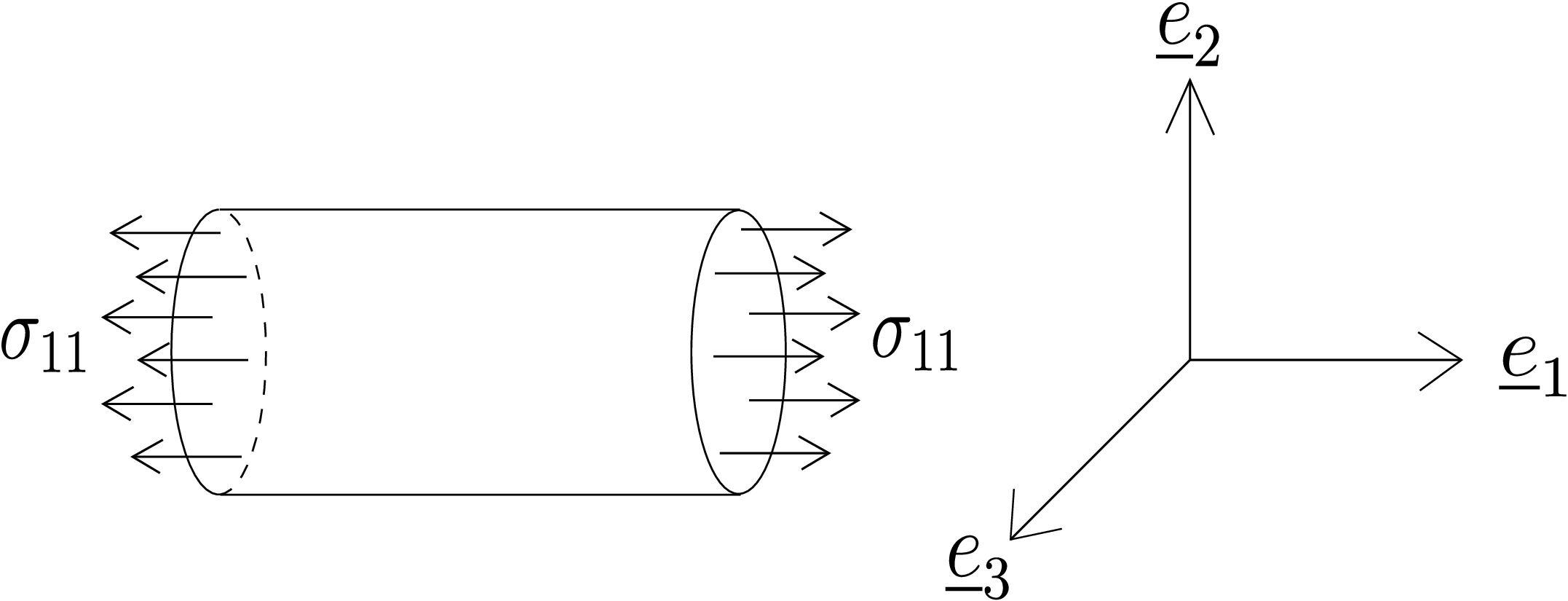
We then increase the value of \(\sigma _{11}\) slowly until the body fails say at \(\sigma _{11}=\sigma _y\). The state of stress at a general point in the body will be \begin {equation} \label {11_simple_tension_state_of_stress} \begin {bmatrix} \sigma _{11} & 0 & 0\\ 0 & 0 & 0\\ 0 & 0 & 0 \end {bmatrix}. \end {equation} The principal stress components for such a state of stress can be obtained directly from the inspection of stress matrix leading to
Thus, the maximum principal stress is simply \(\sigma _{11}\) which should be less than or equal to the critical value of principal stress, i.e., \(\sigma _y\) which we obtained from direct measurement in simple tension test. For a general loading scenario, one has to first obtain the distribution of stress in the body and then obtain the maximum principal stress at every point in the body, say \(\lambda _1(\underline {x})\). One further computes the maximum value of \(\lambda _1(\underline {x})\) among every point in the body and compare it with the critical value \(\sigma _y\) to check for failure, i.e., \begin {equation} \max _{\underline {x}}\lambda _1(\underline {x})<\sigma _y. \end {equation}
We again do the simple tension test to find out the critical value of shear stress in the body. We increase the distributed load \(\sigma _{11}\) as shown in Figure 11.2. The load at which the body fails is \(\sigma _y\). The state of stress is given in \eqref{11_simple_tension_state_of_stress} whose principal stress components are \(\lambda _1=\sigma _{11}\), \(\lambda _2=0\) and \(\lambda _3=0\) as derived earlier. Thus, the maximum shear stress which is obtained by \(\frac {\lambda _1-\lambda _3}{2}\) turns out to be \(\frac {\sigma _{11}}{2}\). This will become equal to the critical shear stress value \(\tau _y\) when \(\sigma _{11}=\sigma _y\) which implies \begin {equation} \tau ^y=\frac {\sigma _y}{2}. \end {equation} Once \(\tau _y\) is obtained through simple tension test, it holds even for general loading scenario. The maximum shear stress for a general loading case with principal stress components \(\lambda _1\), \(\lambda _2\) and \(\lambda _3\), is given by \(\frac {\lambda _1-\lambda _3}{2}\). So, to avoid failure, the following condition should be satisfied at every point in the body: \begin {equation} \frac {\lambda _1-\lambda _3}{2}<\frac {\sigma _y}{2}. \end {equation} We can also obtain the critical value of shear stress \(\tau _y\) from torsion test instead of tension test. Figure 11.3 shows a circular beam subjected to
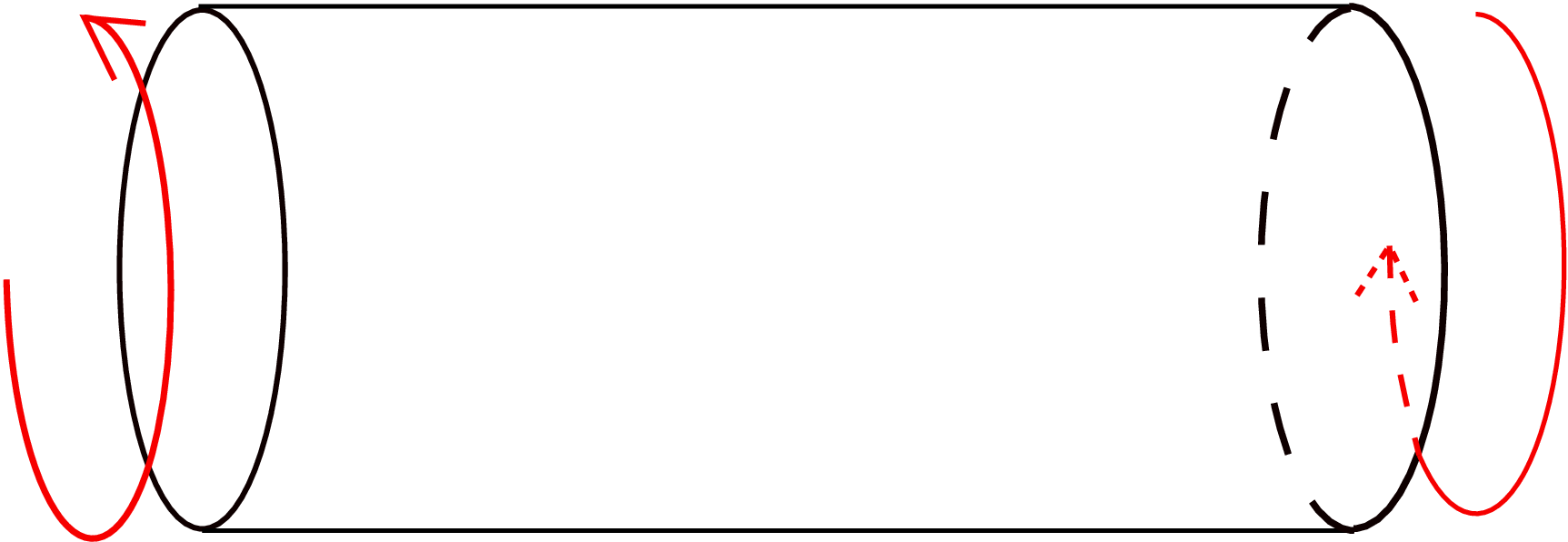
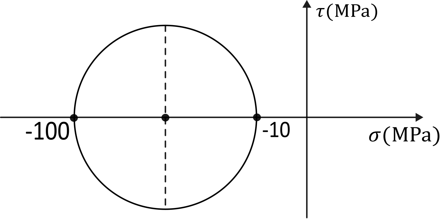
equal and opposite torques at the ends. We had found the state of stress for such a case earlier. In cylindrical coordinate system, the stress matrix can be written as \begin {equation} \label {11_torison_test_state_of_stress} \begin {bmatrix} \underline {\underline {\sigma }} \end {bmatrix}= \begin {bmatrix} 0 & 0 & 0\\ 0 & 0 & \tau _{\theta z}\\ 0 & \tau _{\theta z} & 0 \end {bmatrix}. \end {equation} We can find the maximum shear stress for this state of stress by drawing the Mohr’s circle. As \(e_r\) is a principal axis, we can draw the Mohr’s circle directly. As \(\sigma _{\theta \theta }\) and \(\sigma _{zz}\) are zero, the center of the circle will be at the origin while the radius of the circle will be the length from origin to \(\tau _{\theta z}\). Figure 11.4 shows this Mohr’s circle.
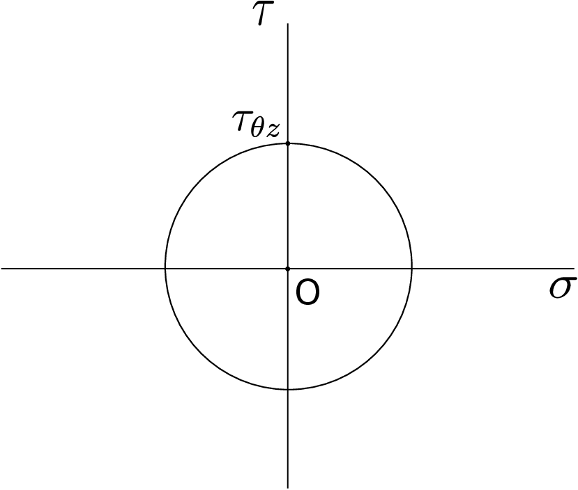
Therefore, the maximum shear stress \(\tau _{max}\) is simply \(\tau _{\theta z}\): the value of shear stress in the cross-sectional plane. We can write this shear stress \(\tau _{\theta z}\) in terms of the applied torque \(T\) as follows:
This happens to be the maximum shear stress at any point for the case of pure torsion. As it changes with radial coordinate \(r\), its maximum value for the entire body is attained when \(r\) is maximum, i.e., on the outer surface of the cylinder. Thus, the critical value of shear stress \(\tau ^y\) can be written as \begin {equation} \tau _y=\tau ^*_{\theta z}=\frac {T^*R}{J}. \end {equation} where \(T^*\) is the critical torque value at failure. Once \(\tau _y\) is obtained from torsion test, for the general loading scenario, one can write \begin {equation} \frac {|\lambda _1-\lambda _3|}{2}<\tau _y=\tau ^*_{\theta z}=\frac {T^*R}{J}. \end {equation} We can also formulate the maximum normal strain and maximum shear strain theories similarly. Let us now look at the distortional energy theory.
Consider a body under general loading. Thus, we have general state of stress at every point in the body. There will be three principal components of stress at every point which we denote by \(\sigma _1\), \(\sigma _2\) and \(\sigma _3\). Let us now obtain the strain components in the principal coordinate system. There is no shear stress in the principal coordinate system and thus the shear strains will also be zero using linear stress-strain relation for isotropic bodies. We only have normal strains \(\epsilon _1\), \(\epsilon _2\) and \(\epsilon _3\) which can be written as follows in terms of principal stress components:
The total stored elastic energy per unit volume will then be
We have to extract the distortional part of energy from this. Remember we had decomposed the stress and strain matrices into hydrostatic and deviatoric (or distortional) parts in an earlier chapter. We can use these hydrostatic parts to obtain volumetric strain energy density, i.e., \begin {equation} \text {Volumetric strain energy/ vol}=\frac {1}{2}\sigma _{vol}\epsilon _{vol} \end {equation} The volumetric stress is simply one-third of the first invariant of stress matrix while the volumetric strain is the trace of strain matrix. Thus
Finally, the distortional energy density can be written as
One can obtain the critical value of distortional energy density from simple tests like tension test or torsion test. In a simple tension test, \(\sigma _2\) and \(\sigma _3\) are zero and we only have \(\sigma _1\). Thus, the distortional energy density for a simple tension test is \(\frac {1+\nu }{3E}\sigma _{11}^2\). Accordingly, the critical value of distortional energy density will correspond to the point where \(\sigma _{11}=\sigma _y\) (the tensile stress value when the body fails), i.e., \begin {equation} \text {Critical distortional energy density}=\frac {1+\nu }{3E}\sigma _y^2. \end {equation} For a general loading scenario, the following condition must be satisfied at each point in the body to avoid failure: \begin {equation} \frac {1+\nu }{3E}(\sigma _1^2+\sigma _2^2+\sigma _3^2-\sigma _1\sigma _2-\sigma _2\sigma _3-\sigma _3\sigma _1)<\frac {1+\nu }{3E}\sigma _y^2. \end {equation} We can similarly do a torsion test to get the critical distortional energy. The stress matrix for a torsion test is given in equation \eqref{11_torison_test_state_of_stress} and the Mohr’s circle for this state of stress is drawn in Figure 11.4. From this, we can find the principal stress components to be
The critical distortional energy from this simple torsion test thus becomes
Accordingly, for a general loading scenario, the following condition must be satisfied at each point in the body to avoid failure: \begin {equation} \frac {1+\nu }{3E}(\sigma _1^2+\sigma _2^2+\sigma _3^2-\sigma _1\sigma _2-\sigma _2\sigma _3-\sigma _3\sigma _1)<\frac {1+\nu }{E}\tau ^{*2}_{\theta z}=\frac {1+\nu }{E}\tau _y^2. \end {equation} We can notice that the expression in the parentheses is proportional to the square of octahedral shear stress \(\tau _{oct}\). Therefore, the distortional energy theory and the octahedral shear stress theory are related.
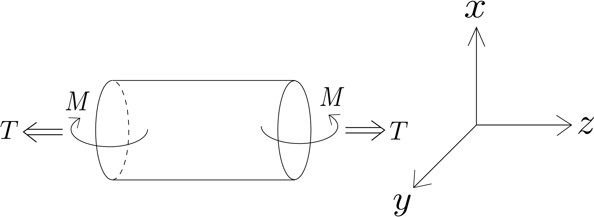
What would be the allowable values of applied torque-moment combination so that the cylinder does not fail? Assume the cylinder obeys the maximum shear stress theory of failure. (NPTEL link)
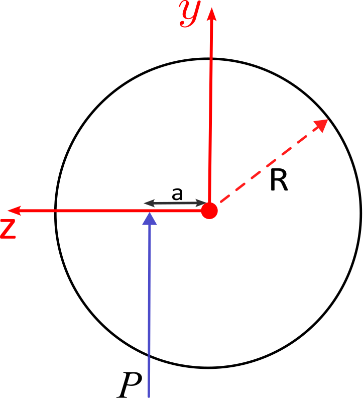
Let us first find the state of stress corresponding to this loading in cylindrical coordinate system. We can consider the effects of bending and torsion separately and then superimpose them. As it is the case of pure bending, we will only get non-zero \(\sigma _{zz}\) due to it as \begin {equation} \label {11_bending_general} \sigma _{zz}=\frac {-My}{I}. \end {equation} Due to torsion, only \(\tau _{\theta z}\) and \(\tau _{z\theta }\) will be non-zero and will be given by \begin {equation} \tau _{\theta z}=\tau _{z\theta }=\frac {Tr}{J}. \end {equation} We now look at the cross-section of the beam as shown in Figure 11.5.
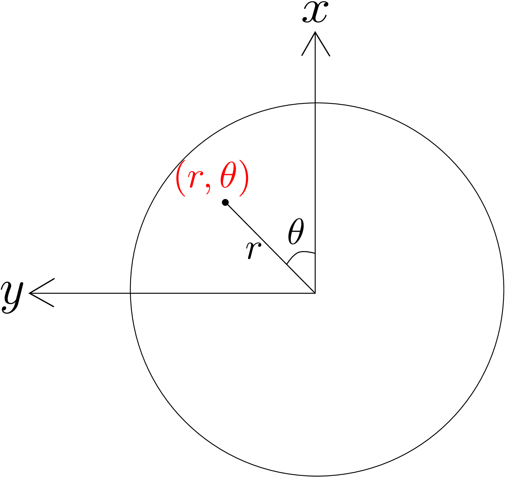
The coordinates of a general point in the cross-section is \((r,\theta )\). Thus, the \(y\)-coordinate of any point is \(r\sin \theta \). Substituting this in equation \eqref{11_bending_general}, we get \begin {equation} \sigma _{zz}=\frac {-M_x\,r\sin \theta }{I_{xx}}. \end {equation} The state of stress obtained by superposition will be \begin {equation} \label {11_example_state_of_stress} \begin {bmatrix} \underline {\underline {\sigma }} \end {bmatrix}= \begin {bmatrix} 0 & \, & 0 & 0\\\\ 0 & \, & 0 & \tfrac {Tr}{J}\\\\ 0 & \, & \tfrac {Tr}{J} & \tfrac {-Mr\sin \theta }{I} \end {bmatrix}. \end {equation} We had also discussed that for circular cross-sections:
Let us now find the maximum shear stress by drawing the Mohr’s circle for the given state of stress. This can be done easily because \(\underline {e}_r\) is already a principal plane. The corresponding Mohr’s circle is shown in Figure 11.6.
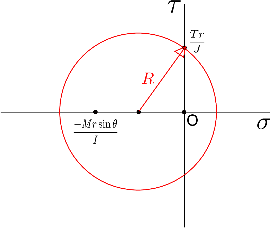
The stress components \(\sigma _{zz}=\frac {-Mr\sin \theta }{I}\) and \(\sigma _{\theta \theta }=0\) are marked on \(\sigma \) axis. The center of the circle is in the middle of these two. Similarly, \(\tau _{\theta z}=\frac {Tr}{J}\) is marked on \(\tau \) axis. The radius is the line joining this point and the center. With the center and radius known, the circle is drawn. From the Mohr’s circle, we can see that the value of maximum shear stress is equal to the radius of the circle, i.e., \begin {equation} \label {} \tau _{max}=\sqrt {\bigg (\frac {Tr}{J}\bigg )^2+\bigg (\frac {Mr\sin \theta }{2I}\bigg )^2}.\nonumber \\ \end {equation} This value must be less than the critical value of shear stress \(\tau _y\) to avoid failure. The body will fail first at the points where the shear stress is maximum. Both the terms in the square root are proportional to the radius. So, the shear stress will be maximum on the outer periphery (lateral surface) of the cylinder where both these terms attain their maximum values. So, we can substitute \(r=R\) in both the terms. Also, the maximum value of \(\sin \theta \) will be 1 at \(\theta =90^\circ \). This is true for points on the \(y\) axis. When we find the points satisfying both the condition, i.e., lying on the periphery as well as the \(y\) axis, we get two points. These points are shown in green in Figure 11.7.
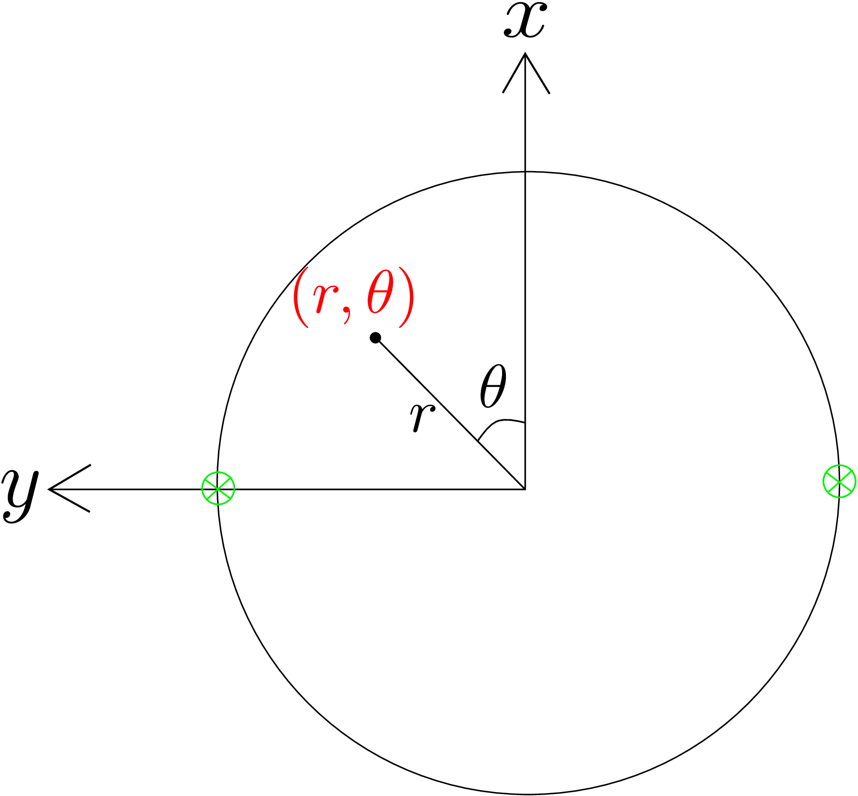
If we can ensure that the shear stress at these points is less than the critical value, the body will not fail. Thus, we can replace \(2I=J\), \(r=R\) and \(\sin \theta =1\) to get the following condition: \begin {equation} \label {11_before_factor_of_safety} \sqrt {\bigg (\frac {TR}{J}\bigg )^2+\bigg (\frac {MR}{J}\bigg )^2}<\tau _y \end {equation} Any combination of bending moment \(M\) and torque \(T\) for which the LHS of the above equation is less than \(\tau _y\) is a safe loading condition for operation. But, in reality, we always design considering some factor of safety for incorporating unexpected circumstances. Suppose the factor of safety to be used in designing is \(N\) which can take any value like 2, 3 or 2.5 but it has to be greater than 1. If the body fails at critical torque \(T^*\) and critical bending moment \(M^*\), the operating torque \(T\) and operating bending moment \(M\) should be such that
Here \(N\) is the factor of safety. Thus, substituting \(T\) by \(TN\) and \(M\) by \(MN\) in equation \eqref{11_before_factor_of_safety}, we get
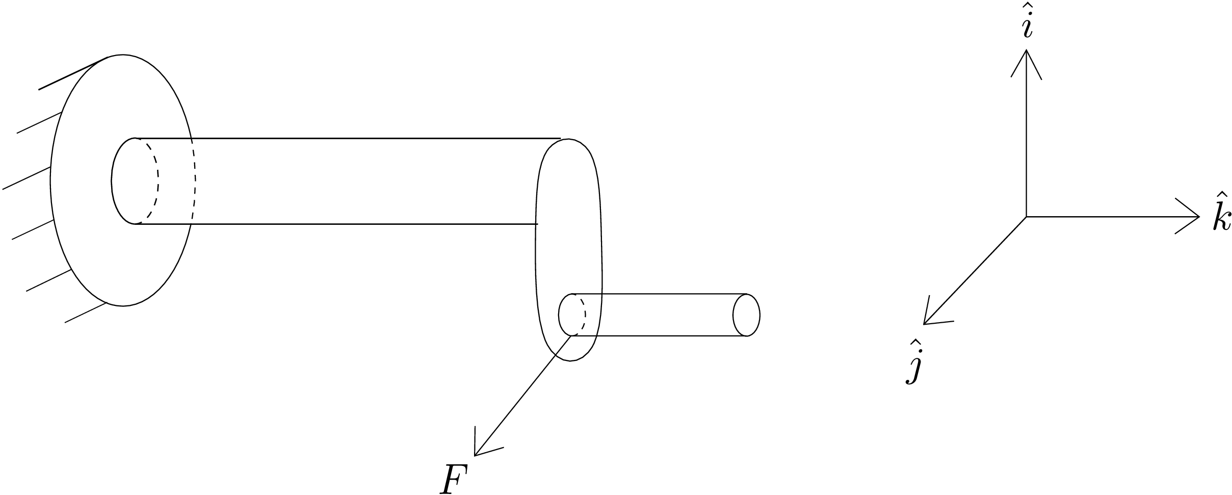
Solution: The applied force can be written vectorially as \begin {equation} \underline {F}=F\hat {j} \end {equation} To design the shaft, we need to find the internal contact force and moment in the shaft’s cross-section. Let us cut a section in the shaft at a distance \(x\) from the clamped end and draw the free body diagram of the right part of the shaft as shown in Figure 11.8.
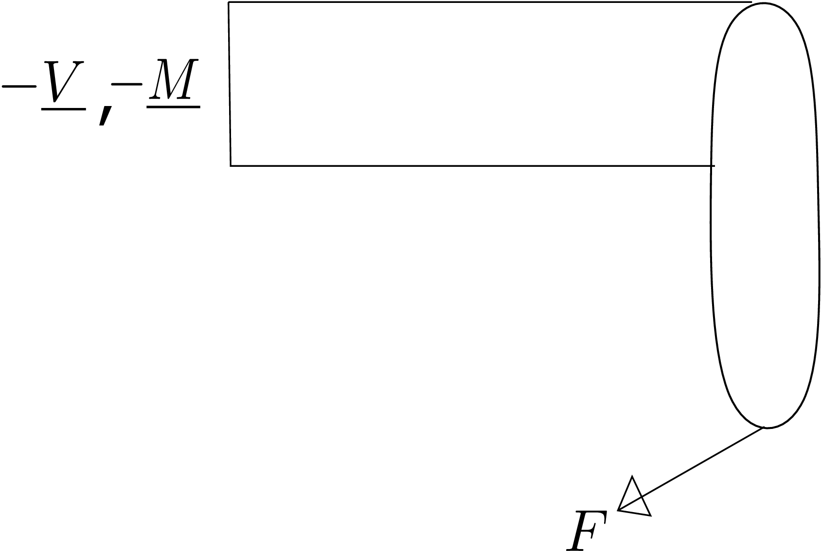
The shear force \(-\underline {V}\) and bending moment \(-\underline {M}\) acts on its left end since its cross-section normal is along \(-z\) axis. Net force balance for the right part of the shaft gives
Let us now do moment balance about the centroid of the left end which yields
The component of moment acting along the axis of the shaft is the torque \(T\) while the other component is the bending moment \(M_x\). As the shear force acts along \(y\) axis, it can be denoted as \(V_y\) such that \(V_y=F\). We now have to find the stress components that generates in the cross-section of the shaft due to these loads. The various non-zero stress components are shown in Figure 11.9a.
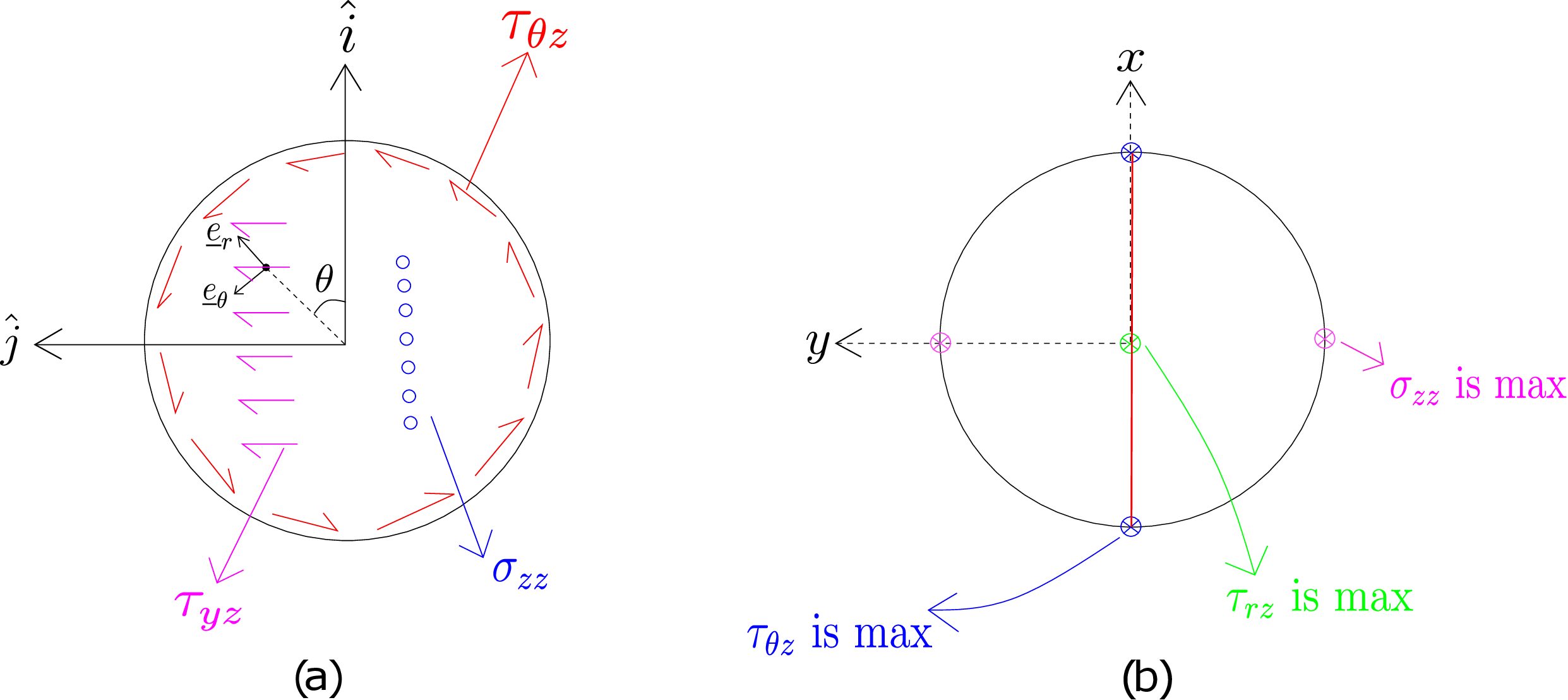
Due to shear force \(V_y\), \(\tau _{yz}\) acts on the cross-sectional plane. The bending moment \(M_x\) generates normal stress \(\sigma _{zz}\) while the
torque generates shear stress \(\tau _{\theta z}\). Their values are given by \begin {equation} \tau _{\theta z}=\frac {Tr}{J},\quad \sigma _{zz}=\frac {-M_x y}{I_{xx}},\quad \tau _{yz}=\frac {V_y Q_y}{I_{xx}t_x}. \end {equation} Here \(t_x=2\sqrt {R^2-r^2\sin ^2\theta }\) is the thickness of the cross-section for points at \(y=r\sin \theta \). All
other variables have usual meaning. The stress matrix for a general point in the cross-section can be obtained by
superposition of all the above stress components. This stress matrix in the cylindrical coordinate system becomes \begin {equation} \begin {bmatrix} \underline {\underline {\sigma }} \end {bmatrix}= \begin {bmatrix} 0 & 0 & \frac {V_y Q_y\sin \theta }{I_{xx}t_x}\\\\ 0 & 0 & \frac {Tr}{J}+\frac {V_y Q_y\cos \theta }{I_{xx}t_x}\\\\ \frac {V_y Q_y\sin \theta }{I_{xx}t_x} & \frac {Tr}{J}+\frac {V_y Q_y\cos \theta }{I_{xx}t_x} & \frac {-M_x y}{I_{xx}} \end {bmatrix}. \end {equation}
Notice that none of the coordinate axes are principal axes. Let us try to use maximum shear stress theory to
design the shaft. The torque and shear force are constant along the length of the beam. Thus, the
stress components \(\tau _{rz}\) and \(\tau _{\theta z}\) do not vary along the length. The bending moment varies with \(x\) and goes
from \(0\) at the right end to maximum at the clamped end. Thus, the bending stress \(\sigma _{zz}\) is maximum at the
clamped end. So, the cross-section at the clamped end is the critical cross-section and failure will occur
first in this cross-section. We thus focus on this cross-section for our analysis which is also shown in
Figure 11.9b. For this cross-section, bending stress \(\sigma _{zz}\) equals \begin {equation} \sigma _{zz}=\frac {yLF}{I_{xx}}. \end {equation} It is just a function of \(y\) and hence it is
maximum at the two points shown in Figure 11.9b. The stress component \(\tau _{rz}\) equals \begin {equation} \tau _{rz}=\frac {FQ_y}{I_{xx}t_x}\sin \theta . \end {equation} Here \(Q_y\) would be
maximum for all points on the line \(y=0\) and \(\sin \theta \) is maximum for \(\theta =90^\circ \). Thus, \(\tau _{rz}\) is maximum at the center of the
cross-section. However, the bending stress is zero at the center of the cross-section. Finally, \(\tau _{\theta z}\) is given by \begin {equation} \tau _{\theta z}=\frac {Tr}{J}+\frac {V_y Q_y\cos \theta }{I_{xx}t_x}. \end {equation} It is
made up of two terms. The first one is maximum when \(r=R\), i.e., on the periphery of the cross-section. The
second term has \(t_{x}\) which is maximum for all points on the \(y=0\) line. Finally, \(\cos \theta \) is 1 at the top and -1 at the
bottom. As \(T=-hF\), the first term has a negative value and likewise the second term should also be negative in
order to maximize the stress component. Thus, we should choose the point where \(\cos \theta \) equals -1. Hence, \(\tau _{\theta z}\)
has maximum negative value at the bottom-most point on \(y=0\) line. We thus note that the three stress
components \(\tau _{\theta z}\), \(\tau _{rz}\) and \(\sigma _{zz}\) attain their maximum values at different points. The point of maximum shear
stress in the cross-section cannot be found using pen and paper - one has to solve it on computer. We
first have to find the principal stress components (\(\lambda _1,\lambda _2,\lambda _3\)) at each point in the cross-section by solving the
eigenvalue problem and then obtain the maximum shear stress as \(\frac {\lambda _1-\lambda _3}{2}\). We then have to find the global maxima
numerically - the point where the maxima is attained would be the critical point from the perspective of
failure.
Notice that even for a very simple design of a shaft/lever, our analysis led to a stress matrix which cannot be
handled using pen and paper. In most practical cases, machines are very complex having multiple parts. Designing
them by hand is indeed impossible and we have to resort to computer programming. This completes our discussion
on theories of failure.