Streamlines, Pathlines and Streaklines
Prapanch Nair
Dept. of Applied Mechanics, IIT Delhi.
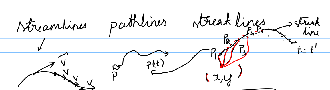
An explainer with an example problem
To appreciate the difference between the three kinds of flow visualization measures we consider the following parametric expression. The velocity field is defined as $\vec{V} = u\hat{i} + v \hat{j} $ where $\hat{i} $ and $\hat{j}$ are both unit vectors in the $x$ and $y$ directions, orthogonal to each other.
$u = \sin t $
$v = 1 $
Streamline.
We know that the streamline $y=f(x) $ is defined as the line whose tangent is in the direction of the velocity vector. For every point in the flow domain, you have a streamline that passes through it, not intersecting with another streamline. For the above example, since velocity components are only dependent on time, at a specific time instance, the velocity will not vary with space. Which means, both $u$ and $v$ are constants representing a uniform flow field at any time instance. Thusthe slope of the streamlines will be a constant at a given time instance. Hence we expect straight lines oriented at a constant angle as the streamlines at a given time instance.
Let's see if we get to visualize that!
For the above example, the slope of the curve at any point would be:
$dy/dx = u/v $
$dy = udx /v $
Integrating the above, we get $y = (1/\sin t)x + C$ We need boundary conditions for the streamlines to get the integration constant $C$. At $x = 0$, let $y=y_s$. Where s is a parameter that remains constant along a streamline and is different from another streamline at the same time instant. applying the boundary condition we get: $C = y_s $ Thus, $ y = (1/\sin t)x + y_s $ is the equation of a streamline. For different y_s values we have different streamline for different y intercepts $y_s$.
Let's now try to plot a few of these streamlines, for different time instance.
# python code
import numpy as np
import matplotlib.pyplot as pl
np.seterr(invalid='ignore')

def y_s(xx,yy,t0):
    y_s  = yy - (1.0/np.sin(t0))*xx
    return y_s

xx,yy = np.meshgrid(np.linspace(0,1.0,25), np.meshgrid(np.linspace(0,1.0,25)))

t0 = np.linspace(np.pi/4.0,np.pi,4)
for i in range(4):
    fig = pl.subplot(2,2,i+1)
    pl.contour(xx,yy,y_s(xx,yy,t0[i]))
    pl.title(r"Time $\pi/$"+str(4-i))
    pl.tight_layout()
pl.colorbar(label="$y_s$")
pl.suptitle("Streamline plots at different time instances", y=1.0)
pl.tight_layout()

As you see, at different times the streamlines are oriented differently, but spatially uniform, as we predicted. And at any time instance, the parameter $y_s$ determines the specific streamline curve (see the line legend).
Pathline
Pathline is obtained by integrating independent coordinates from the velocity expressions.
$\frac{dx}{dt} = u = \sin t$
We integrate with the limits that at $t=0$, the fluid element is at $(x_0,y_0)$ and we integrate until a time value T to get the path the element traverses.
$\int_{x_0}^{X} dx = \int_0^T \sin t dt $
$X- x_0 = -\cos T + 1$
By replacing the variables with smaller case
$x = x_0 +1 -\cos t$
Similarly, $ y = y_0 + t $
The equation of the curve, after removing the parameter $t$ is: $ y = y_0 + \cos^{-1} (-x+x_0+1)$
Lets plot the path lines corresponding to elements at different $(x_0,y_0)$ at time 0, traversed until a time t=1.
def path(x, x_p, y_p):
    y = y_p + np.arccos(-x +x_p+1)
    return y

x = np.linspace(0,1.0,100)
#at t = 0, the initial positions are generated at random
x_0 = np.random.rand(4)
y_0 = np.random.rand(4)
pl.plot(x, path(x,x_0[0],y_0[0]),'r-')
pl.plot(x_0,y_0,'ko')
pl.plot(x, path(x,x_0[1],y_0[1]),'b-')
pl.plot(x, path(x,x_0[2],y_0[2]),'g-')
pl.plot(x, path(x,x_0[3],y_0[3]),'m-')
pl.title("Pathlines for the given velocity field from random points at t=0")

The above code block can be rerun to pick a different set of 4 points and we see how the particles marked by the black dot would move with time showing the corresponding path line.
It may be a good idea to plot the path lines for multiple particles that pass through the same point, lets say (0.01106655,0.03922218) but at a times later than 0. We do this because it is extremely difficult to follow a fluid element in an experiment. Instead we use flow visualizations such as hydrogen bubbles etc. The profile of the bubbles simply map all the particles that once traversed through the source of the bubble.
To do this we integrate the path line as above, with varying limits. At $t=t_1$, $x=x_1$.
$\int_{x_1}^{X} dx = \int_t1^T \sin t dt $
As an example, let's set $t_1=0.5$
$X- x_0 = -\cos T + \cos (0.5) $
$ y - y_0 = T - 0.5 $
We can eliminate T in both as follows:
$ \cos T = \cos (0.5) - X + x_0$
and get the equation of a pathline that passed through the same $p =(x_0,y_0)$ but at a different time instance $t_1$ . $ y = y_0 + \cos ^{-1} (\cos (0.5) - X + x+0) -0.5 $
Now this can be generalized and the pathlines for several particles that passed through the same $p$ but at different times can be plotted as follows.
def path_diffT(x, x_p, y_p,t):
    y = y_p + np.arccos(np.cos(t)-x +x_p) -t
    return y


x = np.linspace(0,1.0,100)
#at t = 0, the initial positions are generated at random
x_0 = 0.01106655
y_0 = 0.03922218
pl.plot(x, path(x,x_0,y_0),'r-',label="passing through p at t=0")
pl.plot(x_0,y_0,'ko')
pl.plot(x, path_diffT(x,x_0,y_0,0.5),'b-', label="passing through p at t=0.5")
pl.plot(x, path_diffT(x,x_0,y_0,0.8),'g-',label="passing through p at t=0.8")
pl.plot(x, path_diffT(x,x_0,y_0,1.0),'m-',label="passing through p at t=1.0")
pl.annotate('p', xy =(x_0, y_0),
                xytext =(0., 1.0),
                arrowprops = dict(facecolor ='green', arrowstyle = "->",),)
pl.legend()

Streakline
Streakline denotes the locus of all points that passed through a given point within a time interval. Let's say the time interval is 0 to T. and we could pick a point from the above example say $p=(0.01106655, 0.03922218)$.
At time t', the expression for pathlines is:
$x_0 = x'-1+\cost' $
$y_0 = y'-t'$
where the prime notation is used to represent a point corresponding to time t'.
We could substitute these values into the expression for pathline itself
$x = x' - 1 + \cos t' +1 - \cos t $
$y = y' - t' + t$
and eliminate $t$
$\cos t = x' + \cos t' - x $
$y = y' - t' + \cos^{-1} ( x' + \cos t' -x)$ or $ \cos t' = x +\cos t -x'$
$y = y' - \cos^{-1}(x + \cos t -x') +t$
This gives us the expression for the streakline.
def path_until_t(x, x_p, y_p, t_s, t):
    x = x_p - np.cos(t) + np.cos(t_s)
    y = y_p + t - t_s
    return x,y

# pathline
xp =  0.01106655
yp =  0.03922218
x = np.linspace(0,1.0,100)
y2 = yp -  np.arccos(x + np.cos(1.0) - xp) + 1.0

#streakline
t = np.linspace(0, 1.0, 30)
#xxx,yyy = path_until_t(x, xp, yp, 0.1,t)

pl.plot(x,y2,'k', label="streak at t = 1, for p ")
pl.plot(xp, yp, 'ro')
pl.plot(x, path(x,xp,yp),'b--', label="path starting at t=0, through p")
pl.plot(path_until_t(x, xp, yp, 0.1,t)[0], path_until_t(x, xp, yp, 0.1,t)[1],'c--', label= "path starting at t=0.1, through p")
pl.plot(path_until_t(x, xp, yp, 0.1,t)[0][-1], path_until_t(x, xp, yp, 0.1,t)[1][-1],'co')
pl.plot(path_until_t(x, xp, yp, 0.2,t)[0], path_until_t(x, xp, yp, 0.2,t)[1],'g--', label= "path starting at t=0.2, through p")
pl.plot(path_until_t(x, xp, yp, 0.2,t)[0][-1], path_until_t(x, xp, yp, 0.2,t)[1][-1],'go')
pl.plot(path_until_t(x, xp, yp, 0.5,t)[0], path_until_t(x, xp, yp, 0.5,t)[1],'m--', label= "path starting at t=0.5, through p")
pl.plot(path_until_t(x, xp, yp, 0.5,t)[0][-1], path_until_t(x, xp, yp, 0.5,t)[1][-1],'mo')
pl.annotate('p', xy =(xp, yp),
                xytext =(-0.1, 0.4),
                arrowprops = dict(facecolor ='green', arrowstyle = "->",),)
pl.xlim(-0.2,0.6)
pl.ylim(-0.5, 1.2)
pl.legend()

The above plot shows the streakline in black and the pathlines of some of the particles with their history. The locus of these points at the current time instance of $t=1$ is clearly the streakline.