In this chapter, we will learn about another important deformation in solid mechanics, i.e., bending of beams. It arises when a beam is subjected to end moments or transverse load. We will analyze beams having both symmetrical and unsymmetrical cross-sections. We will also learn about the shear center of a beam’s cross-section.
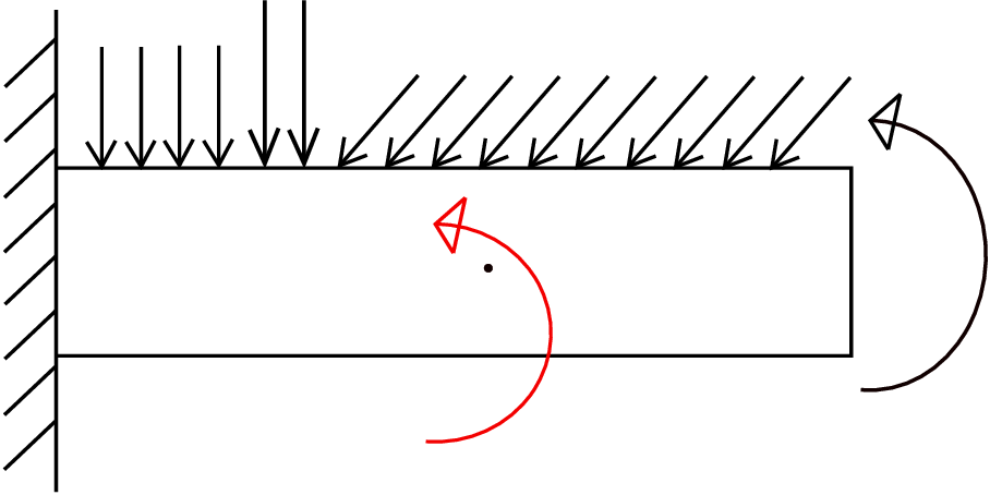
You may have come across problems on beams subjected to terminal transverse load, bending moment or distributed load in your first year mechanics course. Figure 8.1 shows a beam subjected to such loadings: there is a distributed load (force per unit length), a terminal moment at the right end and also a couple at an internal point in the beam.
You may have learnt how to draw shear force and bending moment diagrams for such cases but assumed the beam to not deform. In this course, we will take another step and learn how beams deform or get curved when they are subjected to such loads. The simplest case to begin with is what is called pure bending of beams (see Figure 8.2). Here we have a rectangular beam
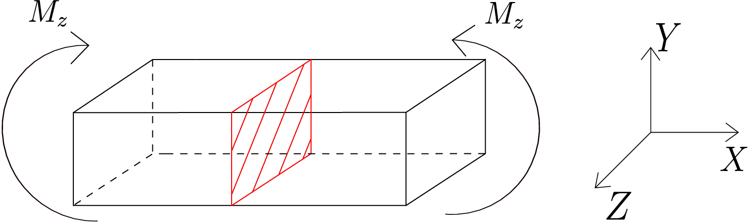
whose axis lies along \(X\) axis. Equal and opposite moments of magnitude \(M_z\) are applied to its end cross-sections in \(Z\) direction, i.e., transverse to the beam. As the total moment on the system is zero, the beam will be in static equilibrium but it also deforms such that it gets curved/bent - see Figure 8.3. Such a deformation is called bending of beams and the applied moment is called bending moment.∗ Let us cut an arbitrary section in the beam as shown in red in Figure 8.2. Using moment balance, we can easily conclude that the internal moment on this section is also \(M_z\). Thus, we have the same internal moment acting on every section of the beam. When the same moment acts on all the beam’s cross-sections without the presence of any internal force, it is called the case of pure bending.
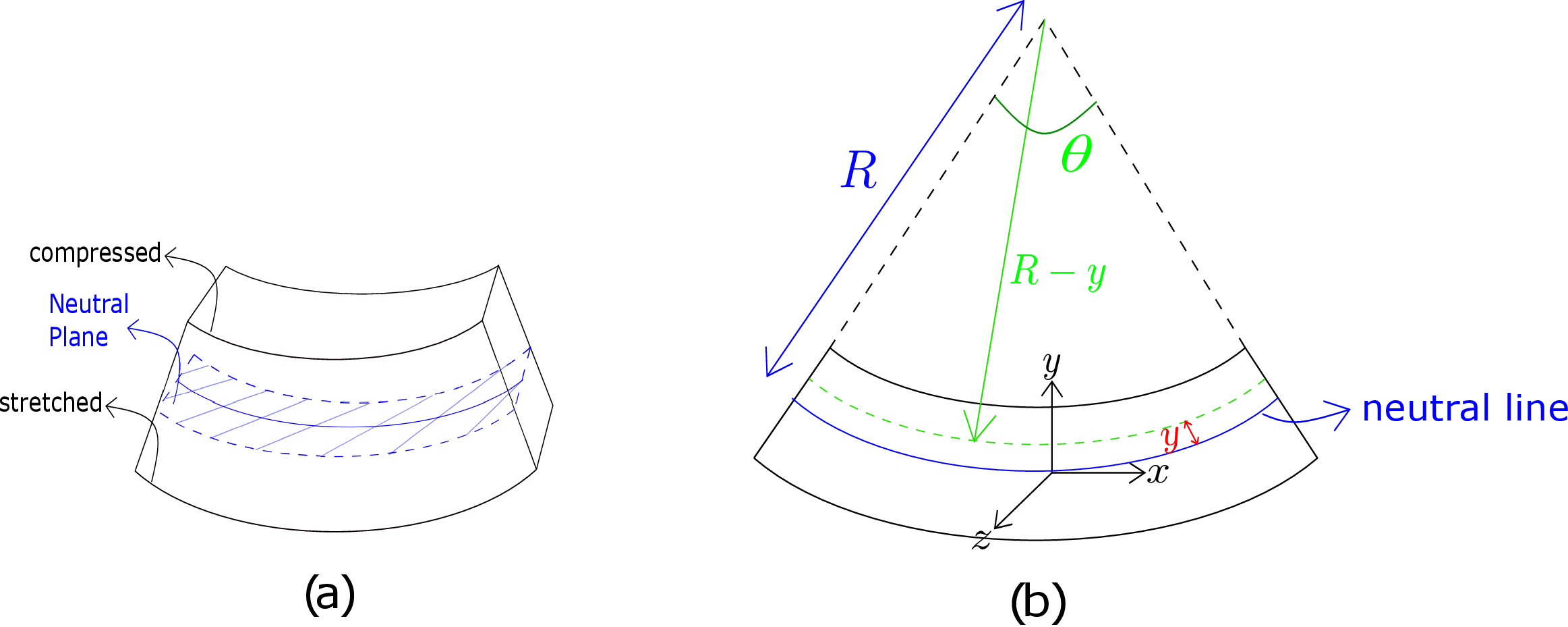
It turns out that in this case, the beam deforms in such a way that all lines of the beam along its length deform into circular arcs as shown in Figure 8.3a. Furthermore, planar cross-sections remain planar after bending. If we imagine this bending deformation, we will note that all the lines parallel to the axis of the beam on its top surface get compressed while those on the bottom surface get stretched. In fact, as we go from the bottom to top surface, the deformation of such lines changes from being stretched to compressed. So, there must be a surface in between whose all such line elements do not undergo any elongation/compression. This surface is called the neutral plane (see the shaded blue plane in Figure 8.3a) as all the axial lines on this plane remain neutral to bending. These line elements on the neutral plane are also called neutral lines.
Let us now find the amount of elongation/compression of these line elements which are parallel to the beam’s axis. We consider a planar view of the beam as shown in Figure 8.3b to simplify the analysis - we assume that the deformation is independent of the coordinate along the width of the beam or \(z\) axis. Just to clarify, the coordinate system is chosen such that \(x\)-axis is along the horizontal line or tangent to the fibers, \(y\)-axis is along the vertical line pointing towards the center of the circle and \(z\)-axis is coming out of the plane. The neutral line is shown as the solid blue line there. It should be noted that we do not know yet the location of this neutral line. Let us consider a longitudinal fiber (shown as a green line) at a distance \(y\) from the neutral line. First of all, we can notice that all these lines, i.e, the green line, the blue line, the topmost and bottom-most longitudinal lines form arcs of concentric circles. If the radius of the circle corresponding to the neutral line is denoted by \(R\) (also called radius of curvature from now on), the radius of the circle corresponding to the green line will be \(R-y\). Let us denote the angle subtended by these arcs at the center as \(\theta \). The length of the the neutral line \(l_{n}\) will be \(R\theta \) which also equals the beam’s undeformed length \(L\) when it was straight, i.e, \begin {equation} \label {8_length_neutral_line} l_{n}=R\theta =L. \end {equation} Similarly, the length of the green line will be
As the undeformed length of all longitudinal lines is \(L\), the longitudinal strain of the green line will be
We have thus obtained longitudinal strain for a general longitudinal line which is at a distance \(y\) from the neutral line. Let us draw the cross-section of the beam as shown in Figure 8.4a.
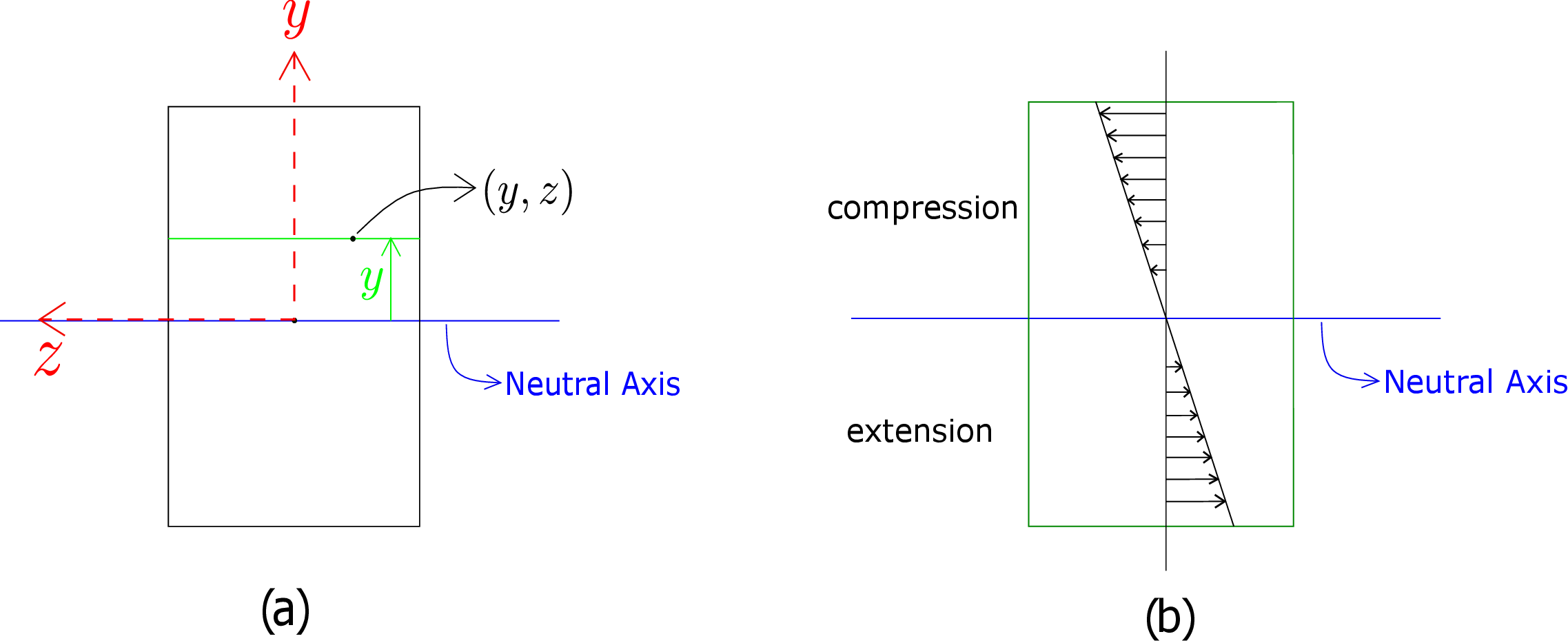
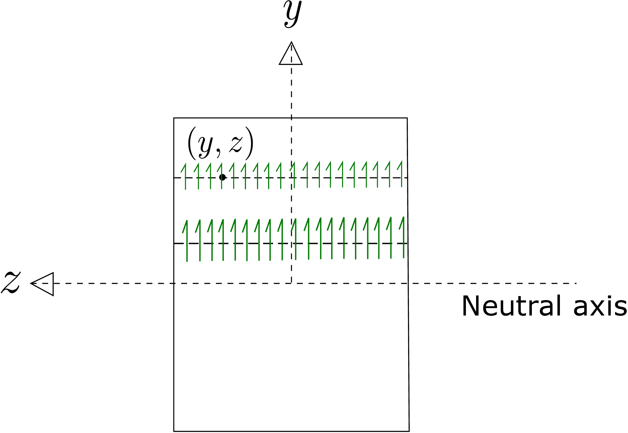
The neutral axis is shown here which is the intersection of the neutral plane with the cross-sectional plane. The green line is shown at a distance \(y\) from the neutral axis. We then consider a general point \((y,z)\) in the cross-section. We found \(\epsilon _{xx}\) to be \(\dfrac {-y}{R}\), i.e., dependent on \(y\) but independent of \(z\). So, any line with a constant \(y\) (like the green line) will have the same \(\epsilon _{xx}\). To obtain \(\sigma _{xx}\), we then use the following stress-strain relationship for isotropic materials: \begin {equation} \label {8_epsilon_xx_relation} \epsilon _{xx}=\frac {1}{E}(\sigma _{xx}-\nu (\sigma _{yy}+\sigma _{zz})). \end {equation} Let us look at Figure 8.2 again. For the case of pure bending, we are only applying moments at the end cross-sections. We are not applying any load on the front, back, top and bottom surfaces. On these surfaces, all components of traction will therefore be zero. Thus, \(\sigma _{yy}\) is zero on top and bottom surfaces while \(\sigma _{zz}\) is zero on front and back surfaces. However, we make an approximation that \(\sigma _{yy}\) and \(\sigma _{zz}\) are zero at all points within the beam too. This is a good approximation because as the beam bends, it is allowed to relax freely in \(y\) and \(z\) directions. Using this approximation in equation \eqref{8_epsilon_xx_relation}, we get \begin {equation} \label {8_sigma_xx_bending} \sigma _{xx}=E\epsilon _{xx}=-E\frac {y}{R} \end {equation} which has been plotted in the cross-sectional plane in Figure 8.4b. Notice that \(\sigma _{xx}\) is compressive above the neutral axis and tensile below it.
In the pure bending scenario, every cross-section only has bending moment acting on it. No net force acts in the cross section. Hence, the integration of \(\sigma _{xx}\) in the cross-sectional plane must vanish, i.e.,
Here \(R\) can be taken out of the integral since it denotes radius of curvature of the deformed neutral line and hence is a constant for the entire cross-section. This reduces the above integral to
The above equation implies that the Y-coordinate of the centroid of the cross-section relative to neutral axis must be zero. Hence, the neutral axis must pass through the centroid of the cross-section. The radius of curvature \(R\) of the deformed neutral line is still an unknown which we find next.
To find \(R\), we first obtain an expression for the moment (about the center of the cross-section) due to internal traction in the cross-sectional plane:
We have already obtained expression of \(\sigma _{xx}\) but we don’t know the variation of \(\tau _{yx}\) and \(\tau _{zx}\) in the cross-sectional plane yet.† Let us just obtain the component of above moment along z axis which we can equate to the externally applied bending moment, i.e.,
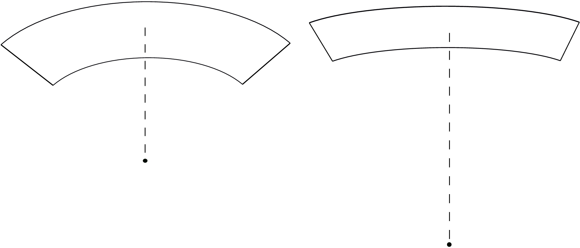
Notice that shear traction components do not contribute to \(M_z\). The integral expression in the above equation is also called the second moment of area about \(z\)-axis and is denoted by \(I_{zz}\). Thus, we finally have \begin {equation} M_z=\frac {E}{R}I_{zz}~\text {or}~ R=\frac {EI_{zz}}{M_z}. \end {equation} The quantity \(\dfrac {1}{R}\) is also called bending curvature and is denoted by \(\kappa \). We can also define a bending modulus as follows: \begin {equation} \label {8_bending_modulus} M_z=\underbrace {EI_{zz}}_{\text {Bending Modulus}}\kappa . \end {equation} Notice that it is the product of the Young’s modulus \(E\) and geometric property \(I_{zz}\). The curvature that gets induced in the beam on application of bending moment is inversely proportional to this bending modulus. If the bending modulus is high, the curvature induced would be smaller which means a large bending moment is required to curve/bend the beam. Note that a larger curvature implies a more curved beam because the radius of curvature is smaller then whereas a smaller curvature represents an almost straight beam because the radius of curvature is large then.‡ This is also demonstrated in Figure 8.5.
We can now rewrite the expression of \(\sigma _{xx}\) in \eqref{8_sigma_xx_bending} after substituting in it the expression of curvature \(\kappa \) from \eqref{8_bending_modulus}, i.e.,
Figure 8.6 shows a rectangular cross section of height \(h\) and width \(b\). The neutral axis is also shown about which the second area moment is to be calculated.
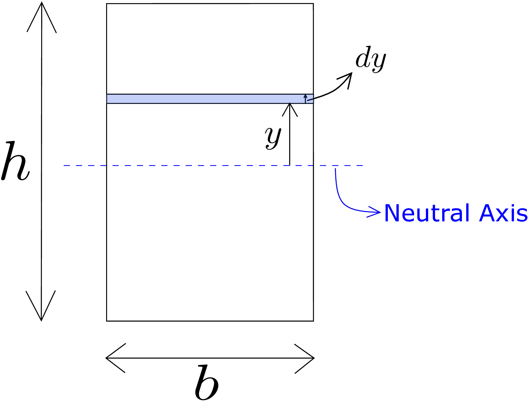
A small rectangular strip of thickness \(dy\) at a distance of \(y\) from the neutral axis is considered. The second area moment about the neutral axis will be
So, \(I_{zz}\) increases with both \(b\) and \(h\) but is more sensitive to \(h\). A small increase in \(h\) brings about a large increase in \(I_{zz}\). We can imagine two rectangular beams made up of the same material and same cross-sectional area (\(bh\)) with the first one having smaller height \(h\) than the second one. Because of larger \(h\), the second beam will have larger \(I_{zz}\) and thus a large bending modulus when compared to the first beam. So, it will be more difficult to bend the second beam although both the beams have the same cross-sectional area.
To find the shape of the deformed cross section, we need to find in-plane normal strains \(\epsilon _{yy}\) and \(\epsilon _{zz}\). Using stress-strain relation, we can write
Here we substituted \(\sigma _{yy}\) and \(\sigma _{zz}\) to be zero as mentioned earlier. Similarly, \(\epsilon _{zz}\) will be
Let us now consider a line parallel to \(y\)-axis in the undeformed cross-section as shown by the green line in Figure 8.7.
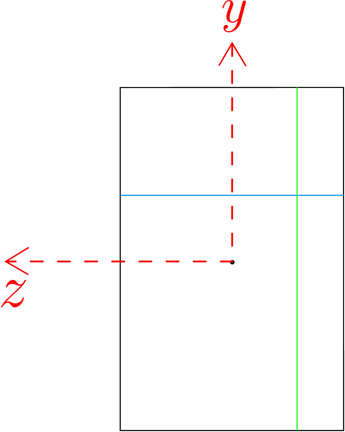
As \(\epsilon _{yy}\) is \(\nu \dfrac {y}{R}\), any point above the neutral axis has positive strain while the corresponding point below the neutral axis will have negative strain of equal magnitude. Thus, upper half of the line drawn parallel to \(y\)-axis will undergo positive longitudinal strain while the lower half will undergo equal but negative longitudinal strain. So, the total length of this line will not change. Now, we consider a horizontal line parallel to \(z\)-axis as shown by the blue line in Figure 8.7. As \(\epsilon _{zz}\) is \(\nu \dfrac {y}{R}\), every point in the blue line will have same \(\epsilon _{zz}\). If these lines are above the neutral axis, they will undergo elongation whereas if they are below the neutral axis, they will undergo compression. Furthermore, this strain being proportional to \(y\), the change in length of such lines will vary linearly. If we draw the deformed cross-section incorporating this effects of \(\epsilon _{zz}\), it will look like the one shown on the right of Figure 8.8, i.e, it becomes a trapezoid.
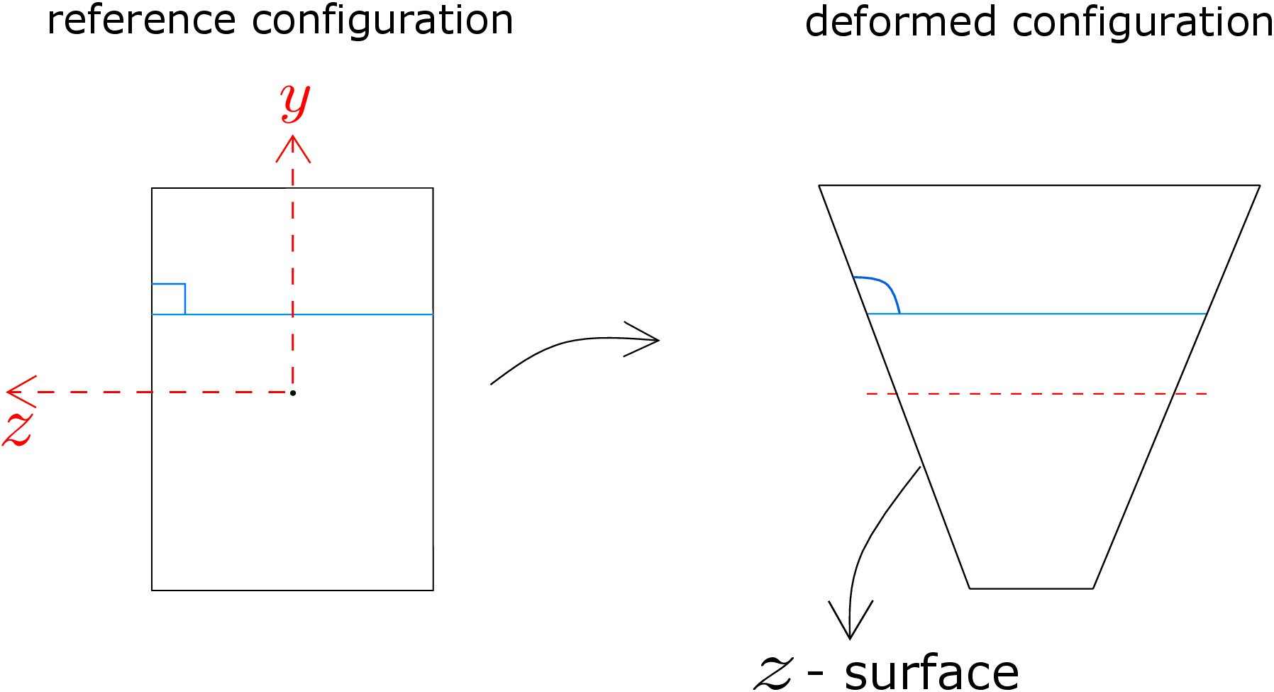
Let us observe the undeformed and deformed configurations in Figure 8.8 more closely: we see that the lines parallel to \(y\)-axis and \(z\)-axis which were perpendicular initially now form an angle greater than \(90^\circ \). This change in angle can happen only if shearing is also taking place. As the angle has increased, we can infer that \(\gamma _{yz}\) is negative. From stress-strain relation for isotropic materials, we know that if \(\gamma _{yz}<0\), then \(\tau _{yz}<0\). Let us consider the two lateral surfaces of the beam with their normals parallel to \(z\) axis. As these surfaces are traction free, all the traction components on the \(z\) surface must be zero including \(\tau _{yz}\). However, if the beam’s cross-section deforms as shown in Figure 8.8, \(\tau _{yz}\) on \(z-\)surface turns out to be non-zero which is a contradiction. Thus, the lines parallel to \(z\)-axis in the beam’s cross-section must also curve along with undergoing change in length. These lines must curve in such a manner that the angle between two infinitesimal lines parallel to \(y\)-axis and \(z\)-axis near the \(z-\) surface remain perpendicular. This will ensure that shear strain and hence shear stress at points on the \(z-\)surface are zero. The curvature of these lines should be such that the lines are convex upward as shown in Figure 8.9.
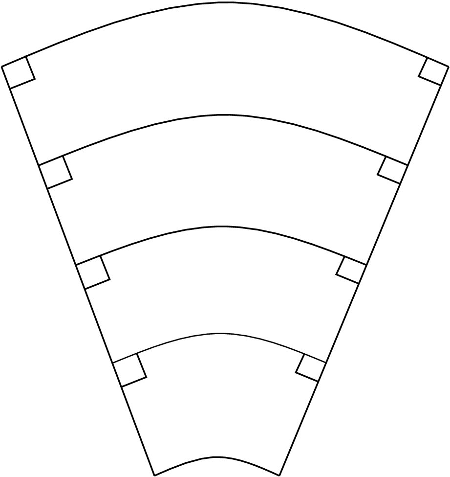
We know that the radius of curvature for the deformed neutral line of the beam is \(R\). If we compare equations \eqref{8_epsilon_xx_bending} and \eqref{8_epsilon_zz_bending}, we can say that the radius of curvature of the centroidal line in the cross-section (coinciding with \(z\) axis) would be \(\dfrac {R}{\nu }\). With this, we can close the topic of pure bending.
In case of pure bending, we had the same moment acting in every cross-section. For this reason, pure bending is also called uniform bending. We will now move on to non-uniform bending of a beam wherein the bending moment is not uniform along the length of the beam. Let us consider a case of loading where we have distributed load \(b(x)\) acting on the beam as shown in Figure 8.10a.
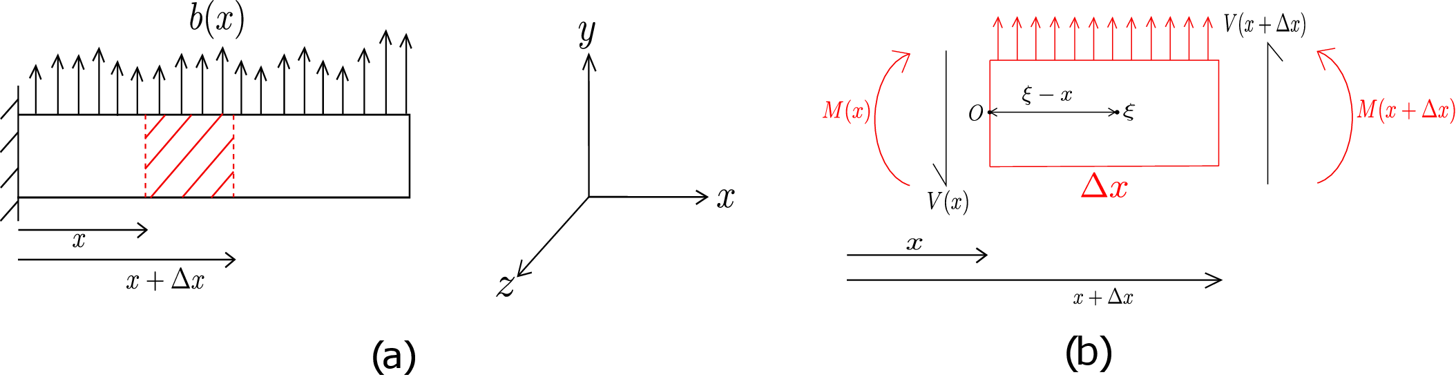
The load \(b(x)\) is assumed to act in \(+y\) direction. Let us cut a small part of the beam of length \(\Delta x\) at a distance \(x\) from the clamped end (see the red region in Figure 8.10a) and further draw its free body diagram as shown in Figure 8.10b. On this small part, apart from distributed load, there will be bending moment as well as shear force acting at the two ends. By convention, for the cross section having normal in \(+x\) direction, shear force acting in \(+y\) direction is considered positive while for the cross section having normal in \(-x\) direction, shear force acting in \(-y\) direction is considered positive. We denote this shear force by \(V\). The center of the left cross-section is marked as \(O\) and the position of a general point in this part of the beam is denoted by \(\xi \) which varies from \(x\) to \(x+\Delta x\). Due to static equilibrium, the net moment on this part of the beam must be zero about any point. In particular, let us do moment balance about \(O\):
As everything is pointing in \(\underline {e}_3\) direction, we obtain the following scalar equation: \begin {equation} M(x+\Delta x)-M(x)+\Delta x ~V(x+\Delta x)+\int _{x}^{x+\Delta x}(\xi -x)b(\xi )d\xi =0. \end {equation} Since this equation holds for an arbitrary part of the beam having length \(\Delta x\), we can divide both the sides by \(\Delta x\) and take the limit \(\Delta x\to 0\) in order to make the beam’s small part reduce to a line, i.e.,
We have derived an important relation between the variation of bending moment and shear force. It says that whenever moment varies along the beam, there has to be a non-zero shear force acting in the beam’s cross-section. The formula for \(\sigma _{xx}\) can still be taken to be the same as earlier. We just have to use the local value of bending moment in the formula, i.e., \begin {equation} \label {8_sigma_xx_bending_1} \sigma _{xx}(x,y,z)=\frac {-M(x)y}{I_{zz}}. \end {equation}
The shear components of traction in the cross-section are \(\tau _{yx}\) and \(\tau _{zx}\). As there is an overall shear force \(V(x)\) acting on the cross section in \(y\) direction, \(\tau _{yx}\) must be non-zero. Let us now try to obtain its distribution in the cross-section. We first make a simplifying assumption that \(\tau _{yx}\) is only a function of \(y\) and not of \(z\). This means that \(\tau _{yx}\) would be the same at all points on lines parallel to \(z\) axis as shown in Figure 8.11 - different horizontal lines will have different \(\tau _{yx}\) though.
To obtain its distribution, we cut a small cuboid element from the beam as shown in green in Figure 8.12a. The bottom surface (\(-y\) plane) of this element is at a distance \(y\) from the neutral plane whereas its left face ( \(-x\) plane) is at a distance \(x\) from the beam’s clamped end. A zoomed view of this green cuboid with all external loads acting on it is shown in Figure 8.12b.
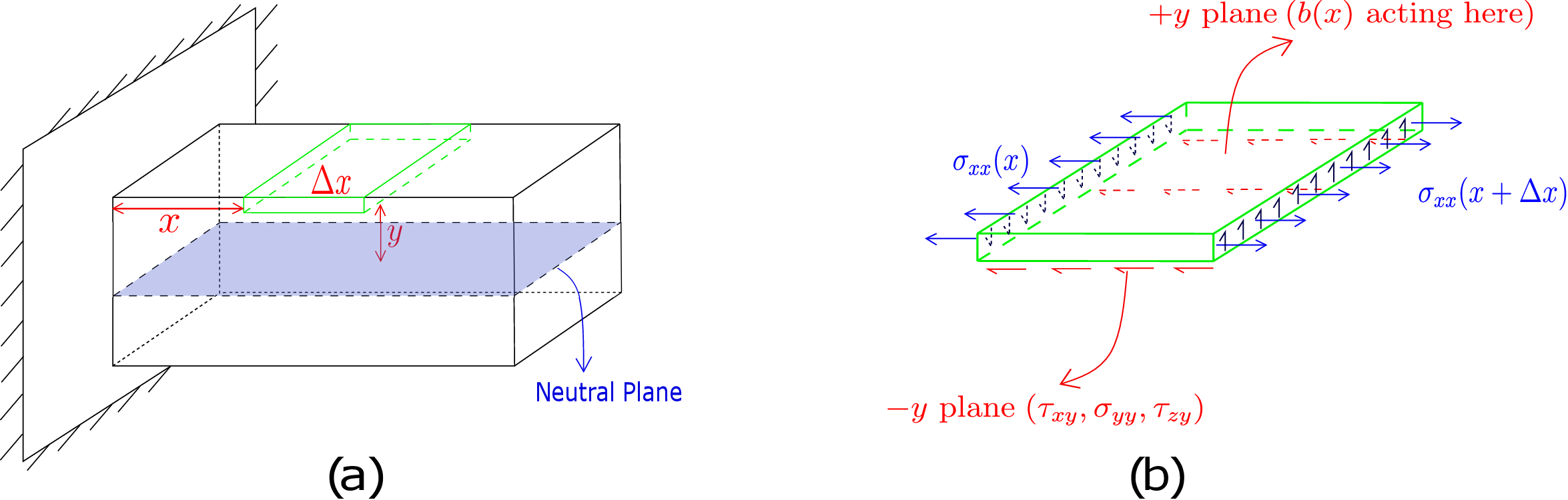
On the top face (\(+y\) plane), distributed load \(b(x)\) acts. The bottom face is the \(-y\) plane and traction components \(\tau _{xy}\), \(\sigma _{yy}\) and \(\tau _{zy}\) act on it in \(-x\), \(-y\) and \(-z\) directions, respectively. The \(+z\) and \(-z\) faces (side faces) are part of the lateral surfaces of the original beam. As external forces are assumed to be applied only on \(+y\)-plane of the beam, the \(+z\) and \(-z\) faces of the element are traction free. On the \(+x\) face, we have bending stress \(\sigma _{xx}\) that we have derived already. We also have \(\tau _{yx}\) and \(\tau _{zx}\) acting there. Similarly, \(\sigma _{xx}\), \(\tau _{yx}\) and \(\tau _{zx}\) act on \(-x\) plane but in negative directions. In order to find \(\tau _{yx}\) (or \(\tau _{xy}\)), we just need to balance the forces on this small cuboidal element in \(x\) direction. The force due to \(\sigma _{xx}\) on \(+x\) and \(-x\) faces is \begin {equation} \int _{\tfrac {-b}{2}}^{\tfrac {b}{2}}\int _{y}^{\tfrac {h}{2}}\sigma _{xx}(x+\Delta x,\eta ,\gamma )~d\eta d\gamma ~~-\int _{\tfrac {-b}{2}}^{\tfrac {b}{2}}\int _{y}^{\tfrac {h}{2}}\sigma _{xx}(x,\eta ,\gamma )~d\eta d\gamma . \end {equation} The force on \(+y\) face has no component in \(x\) direction since the external distributed load acting there is assumed to act in \(y\) direction. However, \(-y\) face has \(\tau _{xy}\) acting on it which contributes the following force in \(x\) direction: \begin {equation} \int _{\tfrac {-b}{2}}^{\tfrac {b}{2}}\int _{x}^{x+\Delta x}-\tau _{xy}(\xi ,y,\gamma )d\xi d\gamma . \end {equation} Summing all the forces in \(x\) direction to zero, we get \begin {equation} \label {force_balance_initial} \int _{\tfrac {-b}{2}}^{\tfrac {b}{2}}\int _{y}^{\tfrac {h}{2}}\Big [\sigma _{xx}(x+\Delta x,\eta ,\gamma )-\sigma _{xx}(x,\eta ,\gamma )\Big ]d\eta d\gamma ~~-\int _{\tfrac {-b}{2}}^{\tfrac {b}{2}}\int _{x}^{x+\Delta x}\tau _{xy}(\xi ,y,\gamma )d\xi d\gamma =0. \end {equation} Upon further substituting \(\sigma _{xx}\) from \eqref{8_sigma_xx_bending_1} in it, we get \begin {equation} \iint _{\text {$x$ plane}}\Bigg [\frac {-M_z(x+\Delta x)\,\eta }{I_{zz}}-\frac {-M_z(x)\,\eta }{I_{zz}}\Bigg ]dA~~-\int _{\tfrac {-b}{2}}^{\tfrac {b}{2}}\int _{x}^{x+\Delta x}\tau _{xy}(\xi ,y,\gamma )d\xi d\gamma =0. \end {equation} As the first integral is over \(x\) plane, \(M_z\) and \(I_{zz}\) act as constants. We had also assumed initially that \(\tau _{xy}\) does not vary with \(z\) or \(\gamma \) coordinate. All these simplifications lead to \begin {equation} -\Bigg [\frac {M_z(x+\Delta x)-M_z(x)}{I_{zz}}\Bigg ]\iint _{\text {$x$ plane}}~\eta dA~~-\int _{x}^{x+\Delta x}\tau _{xy}(\xi ,y)d\xi ~\int _{\tfrac {-b}{2}}^{\tfrac {b}{2}} d\gamma =0. \end {equation} Since the above equation holds for cuboid elements of any length \(\Delta x\), we first divide it by \(\Delta x\) and then take the limit \(\Delta x\to 0\), i.e.,
The integral in the first term above is the y-moment of the \(x\)-face of the cuboid element which is also shown as the shaded area in Figure 8.13a.
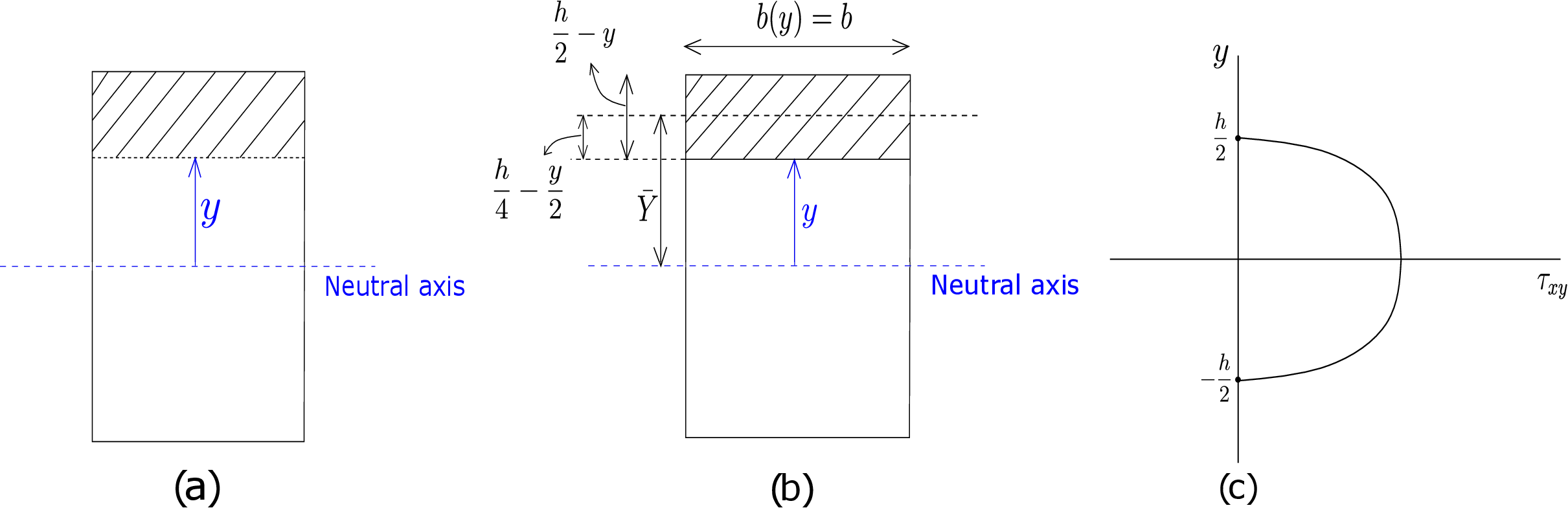
We denote this moment by \(Q(y)\): a function of \(y\) alone. Thus, the final expression for \(\tau _{xy}\) becomes \begin {equation} \label {8_tau_xy_bending} \boxed {\tau _{xy}(x,y)=\frac {V(x)Q(y)}{I_{zz}~b(y)}} \end {equation} which is same as \(\tau _{yx}\): the shear component in the cross-sectional plane. Here, we have allowed \(b\), the width of the cross section, to vary with \(y\). If we compare equations \eqref{8_sigma_xx_bending} and \eqref{8_tau_xy_bending}, we see that while bending stress \(\sigma _{xx}\) is proportional to moment, shear stress \(\tau _{yx}\) is proportional to shear force.
A typical rectangular cross section is shown in Figure 8.13b and we want to find the value of \(\tau _{yx}\) at a distance \(y\) from the neutral axis. For applying equation \eqref{8_tau_xy_bending}, we need to find \(Q(y)\), \(b(y)\) and \(I_{zz}\). As this is a rectangular cross section, width \(b(y)\) is a constant and equal to \(b\). We have already derived \(I_{zz}\) for a rectangular cross section (see equation \eqref{8_Izz_rect}). We thus only need to obtain the expression of the first moment \(Q(y)\) of the area above \(y\) line where \(\tau _{yx}\) is to be calculated (shown as the shaded region in Figure 8.13b). The first moment will simply be \(y\) coordinate of the centroid of the shaded area multiplied by the shaded area. As the height of the shaded area is \(\dfrac {h}{2}-y\), its centroid will be at half of this distance from the \(y\) line and hence at \begin {equation} \bar {Y}= y+ \frac {1}{2}(\dfrac {h}{2}-y)=\frac {1}{2}\bigg (y+\frac {h}{2}\bigg ) \end {equation} from the neutral axis. Thus \(Q(y)\) becomes
which leads to
As \(V\) is the total shear force on the cross section and \(bh\) is the area of the cross section, \(\dfrac {V}{bh}\) equals average shear stress \(\tau _{\text {avg}}\) while \(\tau _{yx}\) at the neutral axis is
Likewise, at the periphery of the cross section \(\bigg (y=\pm \dfrac {h}{2}\bigg )\), we have
This variation of \(\tau _{yx}\) vs \(y\) is shown in Figure 8.13c. We observe that shear stress is maximum on centroidal line and vanishes at the two ends. There is another way to realise the vanishing of shear stress at the ends. The points \(y=\pm \dfrac {h}{2}\) also lie on top and bottom surfaces of the beam, respectively. There is no external traction on the bottom surface whereas on the top surface, the distributed load \(b(x)\) acts in \(y\) direction. Thus, \(\tau _{xy}\) is zero at both top and bottom surfaces. However, due to \(\tau _{xy}\) and \(\tau _{yx}\) being equal, shear stress \(\tau _{yx}\) vanishes at \(y=\pm \dfrac {h}{2}\) in the cross-sectional plane.
In the derivation for rectangular beams, we had assumed that \(\tau _{yx}\) is independent of \(z\)-coordinate. For a circular beam however, this assumption does not hold which we now show. If \(\tau _{yx}\) is constant along lines parallel to \(z\) axis, the shear stress will be as shown in Figure 8.14. Basically, it is non-zero even at the ends.
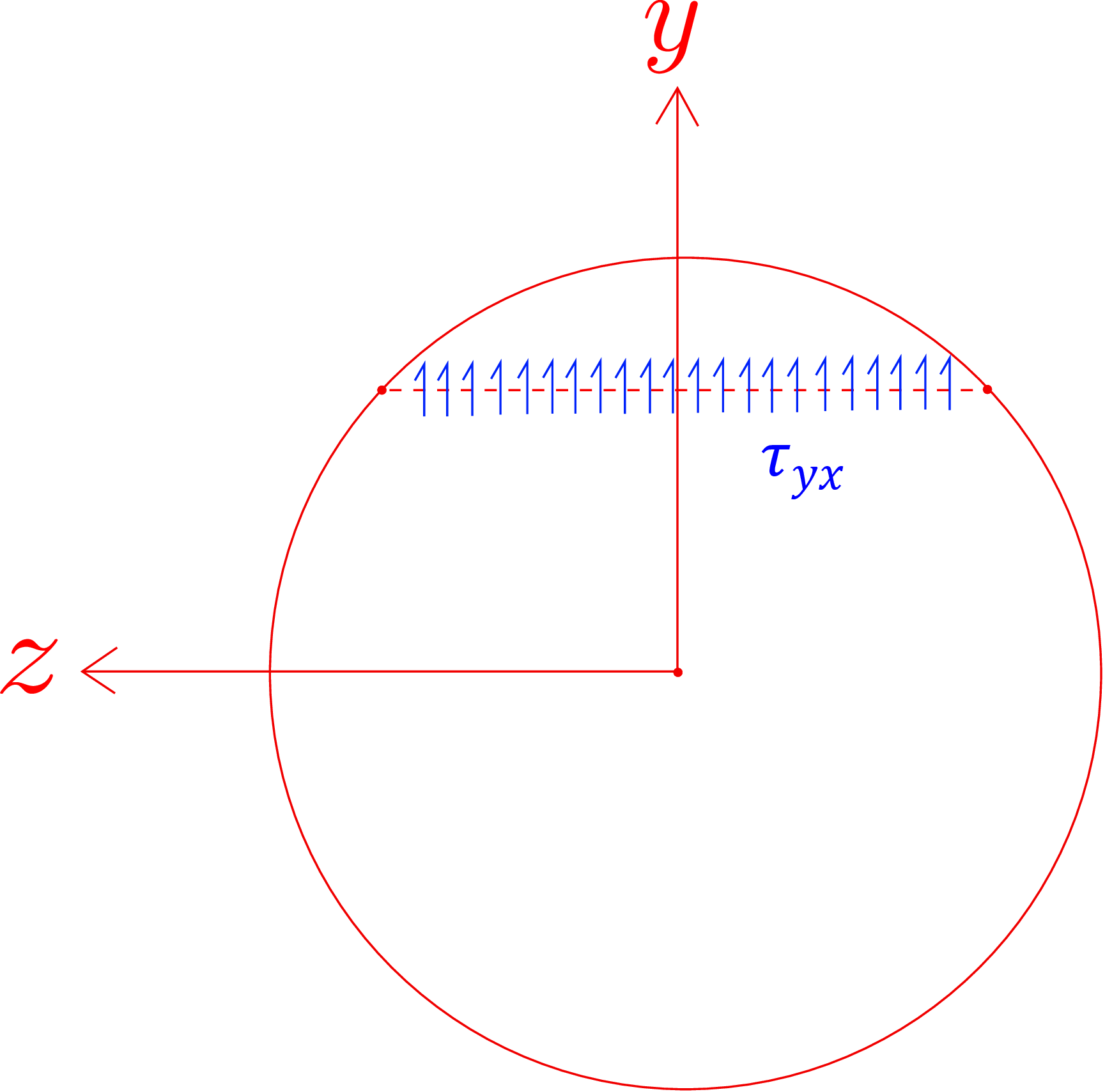
Let us assume a vertical distributed load is acting on the beam’s lateral surface which is also a radial plane for circular beams. Hence, the shear component of traction on the lateral surface along the cylindrical axis will be zero. So, due to symmetry of stress matrix, the radial component of shear traction on peripheral points of cross-sectional plane must also vanish. However, if we look at Figure 8.14, the assumption of \(\tau _{yx}\) being independent of \(z\)-coordinate leads to a non-zero radial component at the periphery which is a contradiction. Thus, we conclude that for circular cross-sections, considering \(\tau _{yx}\) to be independent of \(z\) is not a good assumption. Nevertheless, this assumption is often used even for circular cross-sections since it gives an approximate distribution of shear stress.
For a moment, recollect bending of symmetrical beams, e.g., a beam having rectangular cross-section with its axis along x-axis and the cross-section’s sides along \(y\) and \(z\) axes. When we applied moment on the beam along z-direction, the neutral axis of the cross-section was simply assumed to be parallel to the direction of applied moment (also see Figure 8.15a).

This assumption is not true in general though. For example, Figure 8.15b shows a typical cross-section of an unsymmetrical beam. The neutral axis for this case turns out to be inclined relative to the direction of bending moment. This is non-intuitive since it means the axis of bending (neutral axis) can be in a direction other than the direction of applied moment. Let us investigate this now.
Think of an unsymmetrical beam with its axis along x-axis as shown in Figure 8.16a.
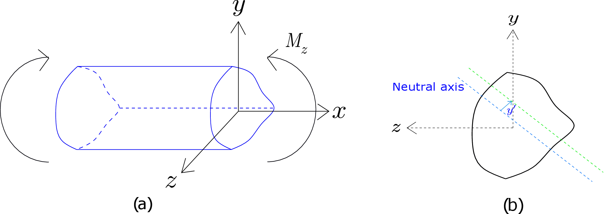
To start with, let us consider the case of pure bending, i.e., equal and opposite terminal bending moments are applied transverse to the beam’s axis. Thus, the bending moment will be constant all along the beam and no shear/axial force will be present in the beam’s cross-section. Figure 8.16b shows a typical cross-section of this beam. As this is the case of an unsymmetrical cross-section, the direction of neutral axis is an unknown too. Let us assume some arbitrary direction (in the plane of the cross-section) for neutral axis which need not pass through the centroid of the cross-section (see Figure 8.16b). The beam bends into a circle of radius \(R\) about the neutral axis. We then think of a line parallel to the neutral axis but at a distance \(y'\) from it (shown by the green line in Figure 8.16b). The longitudinal strain \(\epsilon _{xx}\) for all points lying on this line will be given by \begin {equation} \label {8_epsilon_xx} \epsilon _{xx}=-\frac {y'}{R} \end {equation} following similar logic as earlier for symmetrical cross-sections. Further assuming \(\sigma _{yy}\) and \(\sigma _{zz}\) to be zero as earlier, \(\sigma _{xx}\) at such points will be given by \begin {equation} \label {8_sigma_xx} \sigma _{xx}=E\epsilon _{xx}=-E\frac {y'}{R}. \end {equation} The axial force in the cross-section will thus be \begin {equation} \iint _{\Omega _0}\sigma _{xx}~dA=-\frac {E}{R}\iint _{\Omega _0}y'dA. \end {equation} However, as no axial force acts on the cross-section in case of pure bending, this implies
Thus, the first moment of the cross-section relative to the neutral axis must be zero which simply means
that the neutral axis has to pass through the centroid of the cross-section. So, just like the case of
symmetrical cross-sections, neutral axis passes through the centroid even for unsymmetrical cross-sections.
We now redraw the cross-section keeping in mind that the neutral axis passes through the centroid as
shown in Figure 8.17a and again consider a point \(A\) at a distance \(y'\) from the neutral axis.
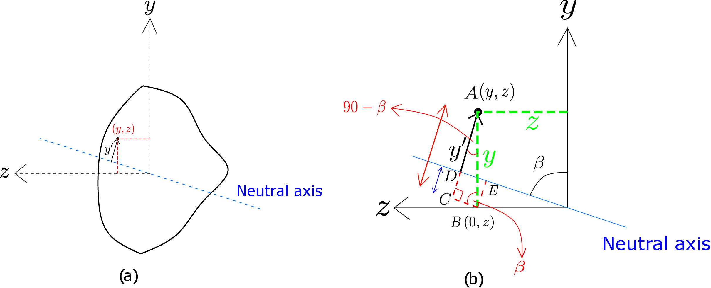
Let the coordinates of this point be \((y,z)\) and express \(y'\) in terms of \(y\) and \(z\). Suppose the neutral axis makes an angle \(\beta \) with the y-axis as shown in Figure 8.17b. Let us construct two lines: one parallel to the neutral axis and passing through the point \(B(0,z)\) while the other one perpendicular to neutral axis and passing through the point \(A(y,z)\) as shown in Figure 8.17b. The point at which these two lines intersect is denoted by \(C\). As the neutral axis makes an angle \(\beta \) with the vertical line, the line \(BC\), constructed parallel to the neutral axis, will also be at an angle \(\beta \) from the vertical line. The other angle (\(\angle BAC\)) in the right triangle \(ABC\) thus becomes \(90^\circ -\beta \). Also, the angle that the neutral axis makes with z-axis will be \(90^\circ -\beta \). Think of another point \(D\) at which the neutral axis and the line \(AC\) intersect. The length \(y'\) will be equal to the difference of the lengths \(AC\) and \(CD\) in Figure 8.17b. We now draw a line perpendicular to the neutral axis starting from point \(B\) and intersecting the neutral axis at \(E\). As \(BCDE\) becomes a rectangle, \(CD=BE\). Thus, we get
Substituting this in equations \eqref{8_epsilon_xx} and \eqref{8_sigma_xx}, we get
Let us now obtain moment about the cross-section’s centroid due to the above normal stress distribution which should equal the externally applied moment, i.e.,
Here \(E\) and \(R\) could be taken out of the integration. Let us define second area moments of the cross-section as follows:
Using them in \eqref{8_moment}, we get \begin {equation} \overrightarrow {M}_{/O}=\frac {E}{R}\Big [\underbrace {(I_{zz}\sin \beta -I_{yz}\cos \beta )}_{M_z}\hat {k}+\underbrace {(I_{yy}\cos \beta -I_{yz}\sin \beta )}_{M_y}\hat {j}\Big ]. \end {equation} So, if the beam has to bend such that the neutral axis makes an angle \(\beta \) from y-axis, the bending moment generated in the cross-section must satisfy
Here \(\kappa \) denotes the bending curvature as earlier. To obtain \(\beta \), we take the ratio of above two equations which yields \begin {equation} \frac {M_y}{M_z}=\frac {I_{yy}\cos \beta -I_{yz}\sin \beta }{I_{zz}\sin \beta -I_{yz}\cos \beta }=\frac {I_{yy}-I_{yz}\tan \beta }{I_{zz}\tan \beta -I_{yz}}.\label {8_general_beta} \end {equation} In the special case when we apply moment about z-axis, i.e., \(M_y=0\), the numerator of the above equation can be set to zero to yield
Furthermore, for cross-sections which are symmetric about \(y\)-axis, the mixed moment of area \(I_{yz}\) vanishes which when substituted in the above equation yields
This means that the neutral axis makes an angle of \(90^\circ \) with the y-axis. In other words, it coincides with z-axis or the direction of applied bending moment something that we had simply assumed earlier. Coming back to the general case for unsymmetrical beams, we can use either of the two equations in \eqref{8_M_z} to obtain bending curvature \(\kappa \). For example, using the former, we get \begin {equation} \label {kappa} \kappa =\frac {M_y}{E(I_{yy}\cos \beta -I_{yz}\sin \beta )}. \end {equation} Finally, substituting \(\kappa \) from the above equation in equation \eqref{8_sigma_xx_2}, we get
Let us consider a special case when y and z axes are aligned with the principal axes of the cross-section but the bending moment acts in an arbitrary direction (see Figure 8.18).
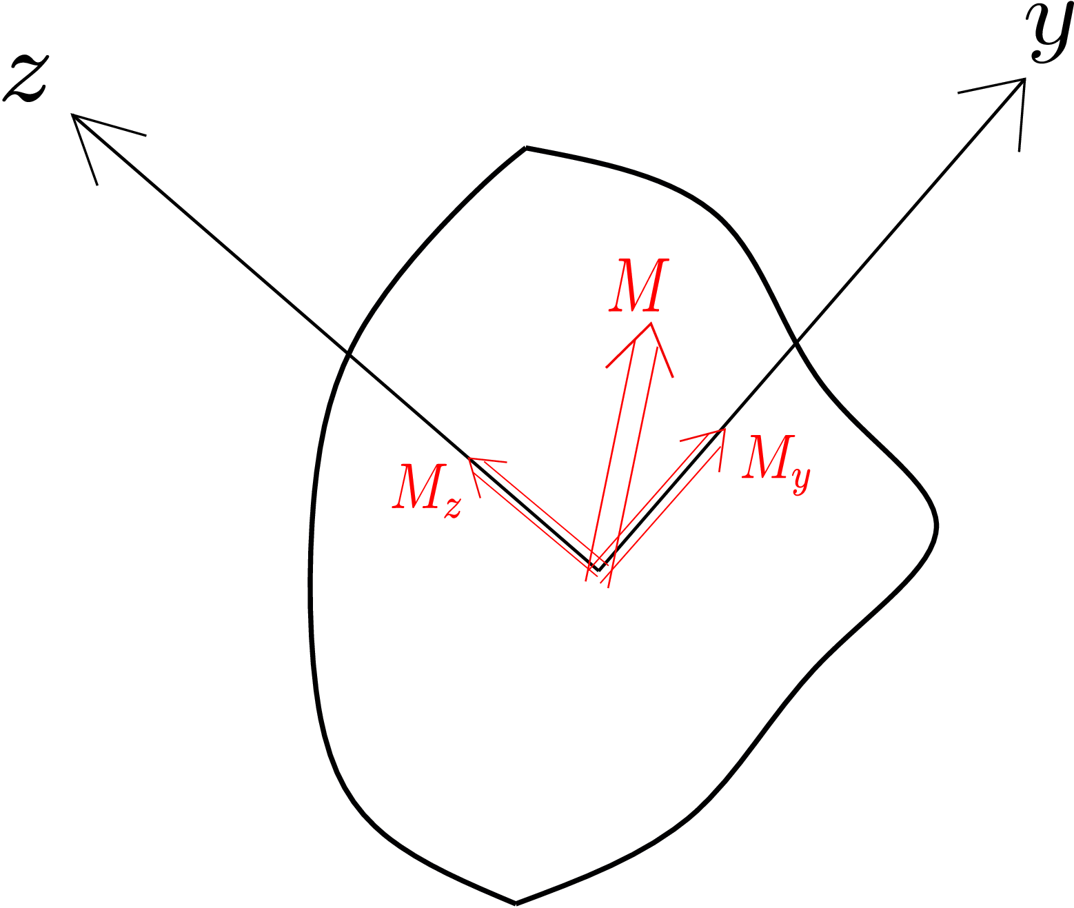
We can resolve this moment along y and z axes as \(M_y\) and \(M_z\), respectively. As y and z axes are principal axes, \(I_{yz}=0\). Substituting this in equation \eqref{8_general_sigma_xx} simplifies it greatly, i.e., \begin {equation} \label {8_principal_axes_formula} \sigma _{xx}=\frac {-M_z y}{I_{zz}}+\frac {M_y z}{I_{yy}}. \end {equation} Furthermore, if we apply moment about z axis only, i.e., \(M_y=0\), we get \begin {equation} \sigma _{xx}=\frac {-M_z y}{I_{zz}} \end {equation} which is the same result that we had obtained earlier for symmetrical cross sections with only \(M_z\) present. We can conclude that if we apply bending moment along the principal axis, the bending happens as if it were a symmetrical cross-section: the neutral axis gets aligned with the direction of applied moment! If we look at equation \eqref{8_principal_axes_formula}, we observe that the first term comes with a negative sign whereas the second term comes with a positive sign. To understand this, consider the cross section shown in Figure 8.19.
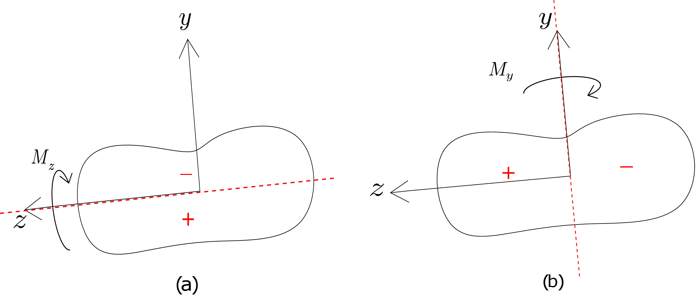
When we apply moment about z axis, the bending is such that the top side (+y side) is under compression whereas the bottom side (-y side) is under tension. Thus, we have a negative sign in front of the first term in equation \eqref{8_principal_axes_formula}. However, if we apply moment about y-axis, the beam bends in such a way that the part of the beam on the left side (+z side) is in tension while the other part is in compression. Since the positive side is in tension, there is accordingly a positive sign in front of the second term in equation \eqref{8_principal_axes_formula}.
In non-uniform bending, a shear force is also present in the cross section due to which the bending moment varies along the length of the beam. The direction of neutral axis is again governed by equation \eqref{8_general_beta}. To obtain shear stress distribution in the cross-section, let us again look at a line which is at a distance \(y'\) from the neutral axis. For symmetrical beams, for simplicity, we had assumed uniform shear stress distribution on lines parallel to neutral axis. If we extend this assumption to unsymmetrical beams, we will have a situation as shown in Figure 8.20a.
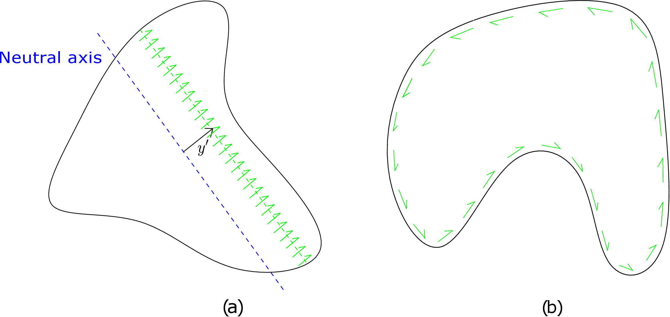
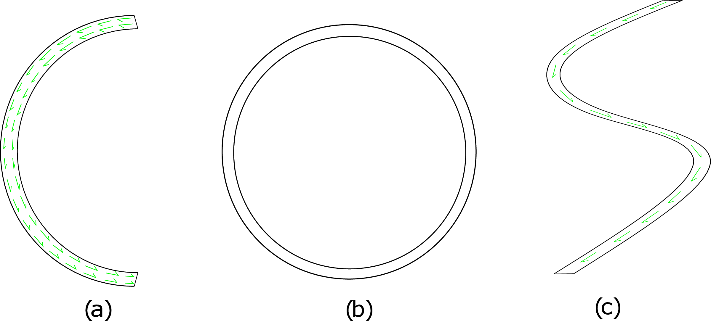
Will such an assumption be valid here? It turns out to be not correct. Whenever we have a beam having symmetrical or unsymmetrical cross-section and its lateral surface is externally loaded in such a way that the external traction has no axial component, then at points along the periphery of the cross-section and on the cross-sectional plane, shear traction has to be directed along the periphery as shown in Figure 8.20b. This is an outcome of the equality of complementary shear stress components. We cannot comment about the direction of shear stress at points away from the periphery though. Accordingly, the derivation of analytical formula for shear stress distribution becomes difficult. However, we can obtain analytical results for special types of cross-sections, i..e, thin and open ones which we discuss now. Figure 8.21 shows three different cross-sections all of which are thin, i.e., their thickness is very small. Figure 8.21b is a closed cross-section while Figures 8.21a and 8.21c are open cross-sections.
We already know that shear stress at points which are close to the periphery of the cross-section has to be
directed along the periphery itself. At points away from the periphery, the direction of shear stress is an
unknown. For thin cross-sections however, the thickness is so small that all points can be safely assumed to
lie near the periphery. Furthermore, there is not enough space for the direction of shear stress to vary
through the thickness. We can thus assume that the shear stress distribution is along the periphery at all
points through the thickness too. In fact, one can also assume the magnitude of shear stress to be uniform
through the thickness owing to the same reason. Later on, we will see why we further want the cross-section
to be open.
Let us consider a general thin and open cross-section beam as shown in Figure 8.22a.
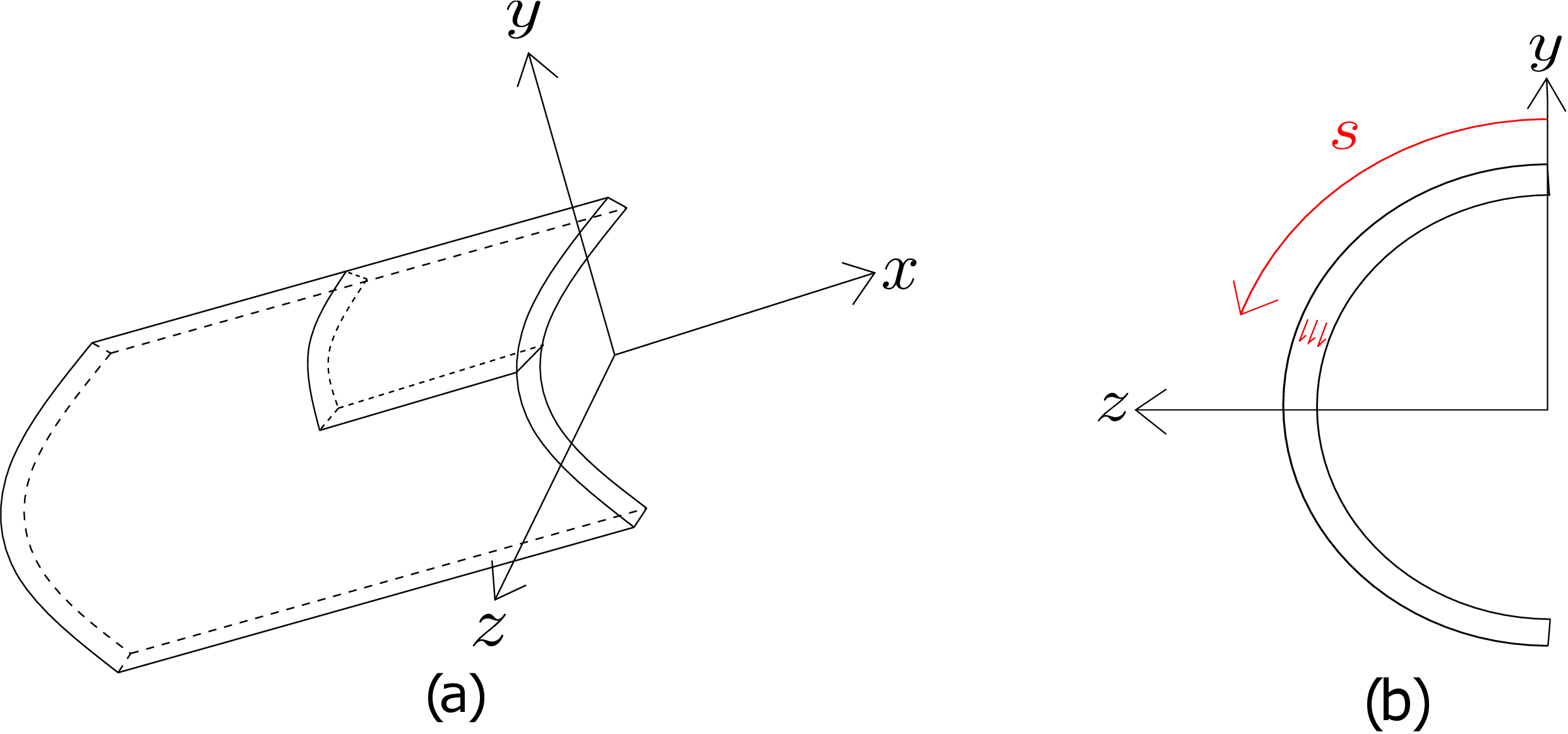
As the shear stress is uniform through the thickness, one can parametrize its distribution using an arc-length coordinate \(s\) running along the cross-section’s periphery as shown in Figure 8.22b. We can further safely assume the shear to flow in the direction of increasing \(s\). If the distribution comes out to be negative in the end, it would simply mean that the shear actually flows in the other direction. We can also denote the shear stress as \(\tau _{sx}\): \(x\) denotes the plane of the cross-section in which shear stress is acting while \(s\) denotes the direction of shear stress. Furthermore, \(\tau _{sx}\) will be a function of \(s\) and \(x\) only. To find \(\tau _{sx}\), we consider a small part of the beam as shown in Figure 8.22a. All the forces acting on this element in x-direction are further shown in Figure 8.23a.
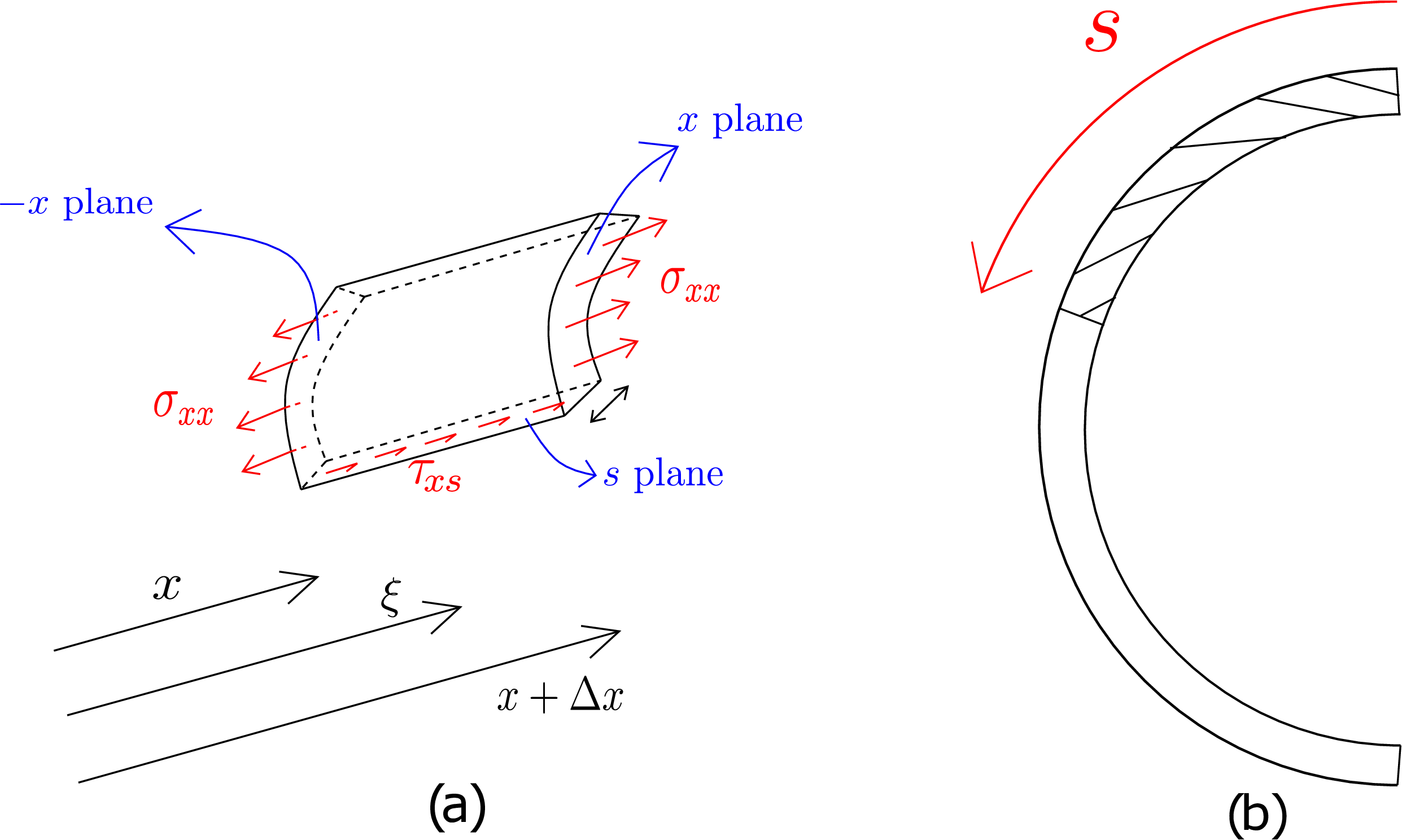
Its end faces (whose normals are in \(s\) direction) will be called \(s\)-faces. On \(+x\) and \(-x\) planes, \(\sigma _{xx}\) acts. The \(-s\) plane at \(s=0\) is traction-free while \(\tau _{xs}\) acts on \(+s\) plane in \(+x\)-direction.§ The total force on this element in x-direction must be zero for equilibrium, i.e., \begin {equation} \iint _\text {x-plane}[\sigma _{xx}(x+\Delta x,y,z)-\sigma _{xx}(x,y,z)]dA+\iint _\text {s-plane}\tau _{xs}(\xi ,s)dA=0. \end {equation} Here \(\xi \) denotes the local coordinate in x-direction which varies from \(x\) to \(x+\Delta x\) for points on \(+s\) face. As the above equation is valid for all beam parts regardless of the size \(\Delta x\), let us first divide the above equation by \(\Delta x\) and then take the limit \(\Delta x \to 0\), i.e., \begin {equation} \lim _{\Delta x\to 0}\iint _\text {x-plane}\frac {[\sigma _{xx}(x+\Delta x,y,z)-\sigma _{xx}(x,y,z)]dA}{\Delta x}+\lim _{\Delta x\to 0}\iint _\text {s-plane}\frac {\tau _{xs}(\xi ,s)dA}{\Delta x}=0.\notag \end {equation} In the second integral above, as the integrand \(\tau _{xs}\) does not vary through the thickness, the integration through the thickness yields \(\tau _{xs}~t_s\) where \(t_s\) denotes the thickness of the cross-section at \(s\). The second area integral thus gets converted into just a line integral along \(x\) leading to
We can now plug in the expression of \(\sigma _{xx}\) from equation \eqref{8_general_sigma_xx} which yields \begin {equation} \label {8_tau_xs_moments_derivative} \tau _{xs}=-\frac {1}{t_s}\iint _\text {x-plane}\frac {M_z'(yI_{yy}-zI_{yz})+M_y'(yI_{yz}-zI_{zz})}{I^2_{yz}-I_{yy}I_{zz}}dA. \end {equation} We can then replace the derivatives of moments with shear forces using the following relations the first of which which we had derived earlier in \eqref{8_Moment_shear_force_relation}:
Upon plugging them into \eqref{8_tau_xs_moments_derivative}, we get \begin {equation} \label {8_before_area_integral} \tau _{xs}=-\frac {1}{t_s}\iint _\text {x-plane}\frac {-V_y(yI_{yy}-zI_{yz})+V_z(yI_{yz}-zI_{zz})}{I^2_{yz}-I_{yy}I_{zz}}dA. \end {equation} As shear forces and second area moments are constants for a cross-section, the denominator of the integrand can be taken out of the integration. We just need to work out the integrals \(\iint ydA\) and \(\iint zdA\) in the numerator. These integrals are over the x-plane of the small element only and not over the entire cross section: see Figure 8.23b which shows the domain of this integration as the shaded region running from arc-length coordinate 0 to \(s\). The integrals \(\iint ydA\) and \(\iint zdA\) over this shaded part of x-plane will give us the first moment of shaded area in \(y\) and \(z\) directions, i.e.,
Here \(\bar {Y}^s\) and \(\bar {Z}^s\) are the centroidal coordinates of just the shaded region. Similarly, \(A^s\) is the area of the shaded region. Upon plugging them into equation \eqref{8_before_area_integral} and further noting that \(\tau _{xs}=\tau _{sx}\), we finally get \begin {equation} \tau _{sx}=-\frac {1}{t_s(I^2_{yz}-I_{yy}I_{zz})}\left [-V_y(Q_y^sI_{yy}-Q_z^sI_{yz})+V_z(Q_y^s I_{yz}-Q_z^s I_{zz})\right ]. \end {equation} This is the general formula for shear stress distribution in thin and open cross-sections. We can again consider the special case where y and z axes are aligned with the principal axes in which case \(I_{yz}\) vanishes. The above formula then simplifies to
If we further assume \(V_z=0\), our formula reduces to \begin {equation} \label {shear_stress_last} \tau _{sx}=-\frac {V_yQ_y^s}{I_{zz}t_s}. \end {equation} This is the same expression that we had derived earlier for symmetrical cross-sections except that there is a negative sign here. This difference arises because the direction of increasing \(s\) that we have chosen here coincides with \(-y\) direction.
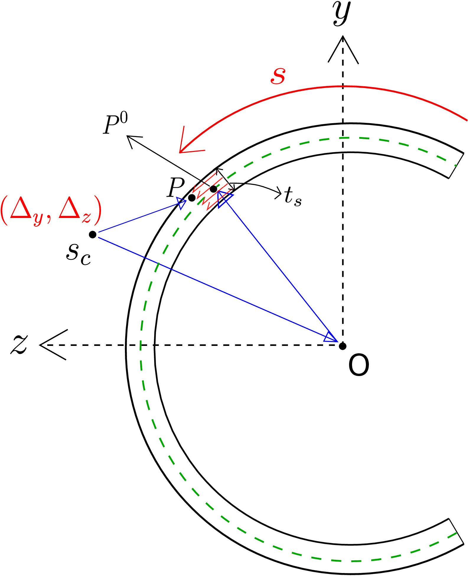
In this section, we will learn about a new concept, i.e., shear center of a cross-section. It is defined as the point in the cross-section relative to which the net torque due to shear stress distribution (originating because of transverse load) vanishes. Obtaining an analytical formula for the location of shear center for a general cross-section isn’t feasible. However, the same can be derived for thin and open cross-sections. We show this derivation now. We had derived the following formula for shear stress \(\tau _{sx}\) at arc-length \(s\): \begin {equation} \label {8_tau_xs} \tau _{sx}=-\frac {1}{t_s(I^2_{yz}-I_{yy}I_{zz})}\left [-V_y(Q_y^sI_{yy}-Q_z^sI_{yz})+V_z(Q_y^s I_{yz}-Q_z^s I_{zz})\right ]. \end {equation} which is assumed to be uniformly distributed through the cross-section’s thickness. Let us denote by \(s_c=(\Delta _y,\Delta _z)\) the location of the shear center as shown in Figure 8.24. The centroid of the cross-section is located at O. As the net torque \(T\) about \(s_c\) vanishes as per definition, we can first find the total moment about \(s_c\) and then equate its x-component to zero. Let us denote the cross-sectional area by \(\Omega \) and an arbitrary point in the cross-section by \(P\). The position vector of \(P\) with respect to shear center (\(\overrightarrow {r_P}_{/s_c}\)) can be written as follows: \begin {equation} \overrightarrow {r_P}_{/s_c}=\overrightarrow {r_P}_{/O}+\underbrace {\overrightarrow {r_O}_{/s_c}}_{-(\Delta _y\hat {j}+\Delta _z\hat {k})}. \end {equation} The total torque \(T\) due to shear stress distribution will thus be
In the second integral term, the shear center position \((\Delta _y\hat {j}+\Delta _z\hat {k})\) can be taken out of the integral while the integral of shear stress over the cross-section gives the total shear force \(\overrightarrow {V}\) in the cross-section. For the first integral, let us write area \(dA\) as \(dsdt\) and change the area integral into two line integrals: one along the arc-length \(s\) and the other along the thickness \(t\). Thus, the above equation can be rewritten as
The expression \(\int _t\overrightarrow {r_P}_{/O}(s,t)dt\) gives us the first moment which we can replace by the position vector of point \(P^0\) times the thickness of the cross-section at arc-length \(s\), i.e., \(t_s\). Here \(P^0\) denotes the centroidal point at arc-length \(s\). These centroidal points form the centerline of the cross-section shown as the dashed green line in Figure 8.24. Thus, we get \begin {equation} \label {8_before_constants} T_{/s_c}=\int _{s=0}^{L_c}t_s(\overrightarrow {r_{P^0}}_{/O}(s)\times \tau _{xs}\hat {s})\cdot \hat {i}\,ds-[\Delta _y V_z-\Delta _z V_y] \end {equation} where \(L_c\) denotes the arc-length along the cross-section boundary and should not be confused with the length of the beam. Upon working out the above integral, we get \begin {equation} T_{/s_c}=C_y V_y+C_z V_z-[\Delta _y V_z-\Delta _z V_y] \end {equation} where \(C_y\) and \(C_z\) are the constants obtained through the integration over the cross-section’s arc-length. As the torque about the shear center must be zero, we get the following upon rearranging:
Furthermore, as this holds for arbitrary \(V_y\) and \(V_z\), we finally obtain
Let us consider the case when only \(V_y\) acts on the cross-section and (y, z) axes are also the principal axes. So, \(I_{yz}\) becomes zero and formula \eqref{8_tau_xs} for \(\tau _{sx}\) simplifies to \begin {equation} \tau _{sx}=\frac {-V_yQ_y^s}{I_{zz}t_s}. \end {equation} Plugging this expression in equation \eqref{8_before_constants}, we get
Thus, we get \(z\)-coordinate of the shear center to be
Proceeding along similar lines, \(y\)-coordinate of the shear center turns out to be
Keep in mind that the above two formulas hold only if \(y\) and \(z\) axes are the principal axes of the cross-section.
We now illustrate that a beam can also twist when subjected to transverse load if the line of action of transverse load does not pass through shear center. We show such a beam in Figure 8.25 which is clamped at one end and a point load is applied in the transverse direction at the other end at point \(A\).
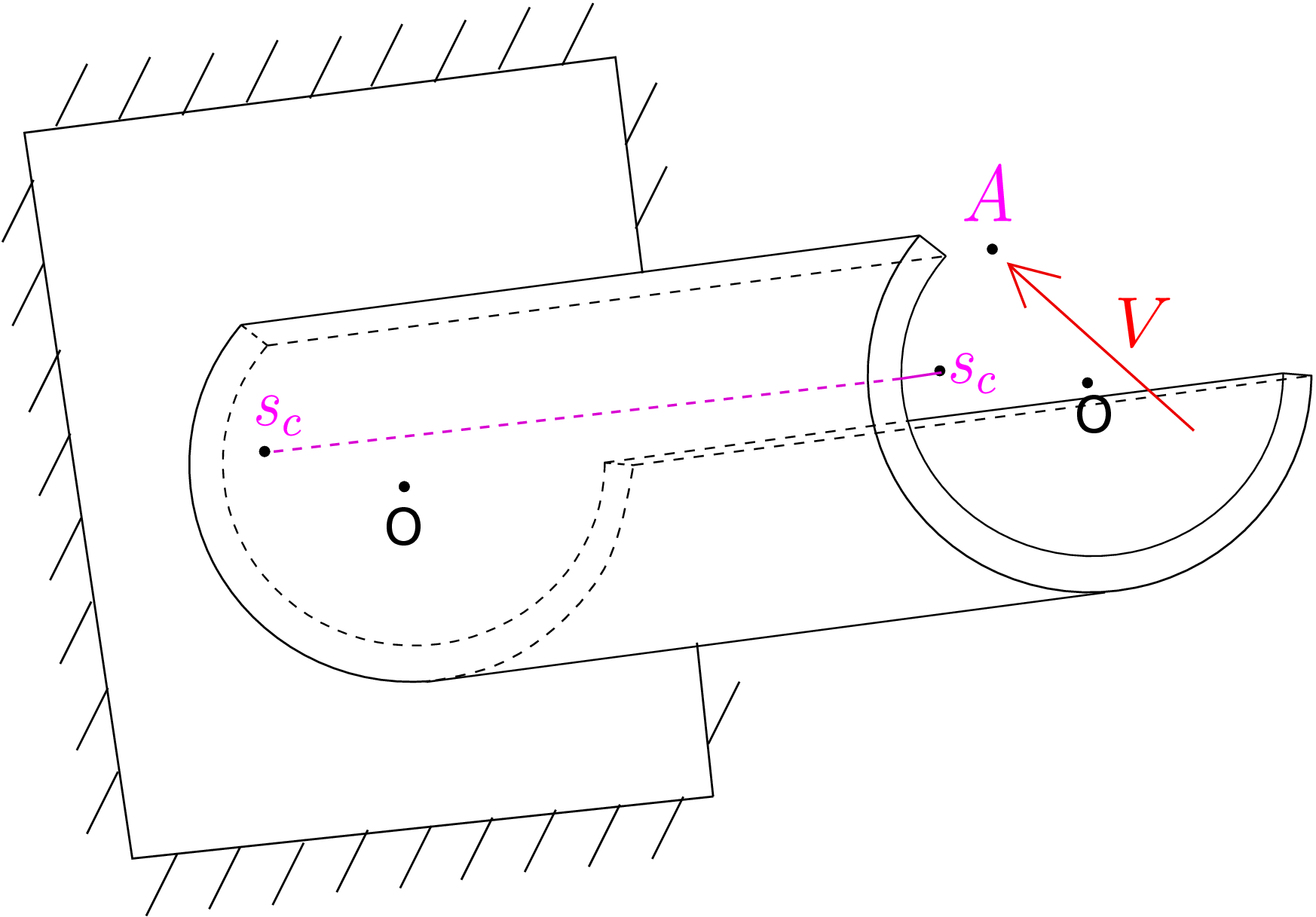
The line joining the shear center of different cross-sections is also shown there. Let us isolate the beam from the clamped end support and draw its free body diagram wherein we also include the reactive shear stress distribution from the clamped support. The net moment on the beam would have to be zero about any general axis in static equilibrium. Consider this axis to be the line of shear centers for which the moment about it would be torque since this axis is perpendicular to the beam’s cross-section. The torque due to shear stress distribution in the left end cross-section about the shear center of the left end cross-section will be zero by the definition of shear center. However, the torque due to the applied transverse load about the axis of shear center will be non-zero since the load is acting eccentrically to the shear center axis. Thus, a net torque acts on the beam which will also induce twist in the beam in addition to the usual bending due to transverse load. This twist will lead to additional reaction of shear stress distribution from the support on the left end cross-section so that the overall torque on the entire beam finally vanishes. Needless to say if we apply the transverse load such that its line of action passes through the shear center at the right end cross-section, there will be no tendency in the beam to twist and the beam will undergo just bending.
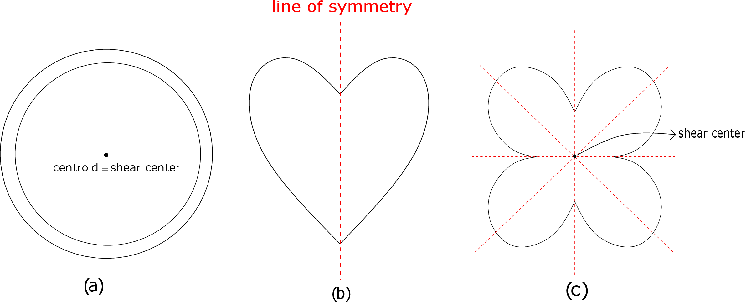
It can be shown using formulas \eqref{8_z_coord} and \eqref{y_coord} for the shear center that it always lies on the line of symmetry of the cross-section (if any present). For example, consider several symmetrical cross-sections in Figure 8.26. In Figure (8.26a), we have an annular cross-section for which all diametrical lines are lines of symmetry. Accordingly, shear center and its centroid coincide. In Figure (8.26b), we have a heart-shaped cross-section which has just one line of symmetry as shown in the figure. Accordingly, the shear center lies on this line. To fix the other coordinate of shear center, one would have to use the formula derived above. Finally, in Figure (8.26c), we have a flower-shaped cross-section having four-fold symmetry. As the shear center must lie on all lines of symmetry, it gets uniquely specified here too just by inspection.
Solution: Composite beams are constructed using more than one material to enhance their strength. In general, the neutral axis of a composite beam will not lie at the geometric centre of the cross-section. Let us suppose that the neutral axis (NA) lies at a distance ‘\(a\)’ from the midline of the cross-section. The bending strain profile will be linear, continuous and pass through zero at the NA as shown below.
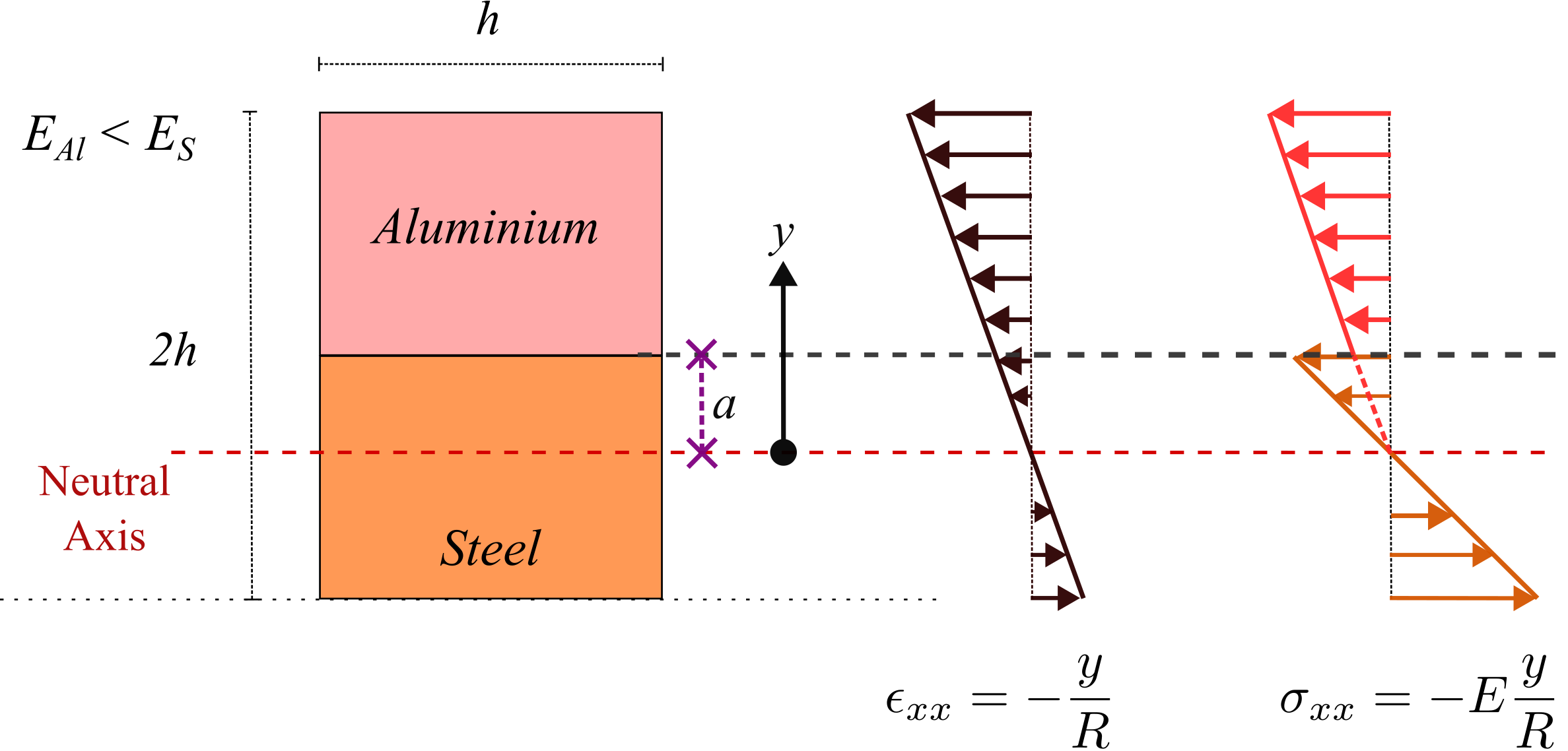
It obeys \(\epsilon _{xx}\;=\;-\dfrac {y}{R}\) where \(y\) is the distance from neutral axis. However, the bending stress profile will be discontinuous at the location where the material changes. It follows the following formula: \begin {align*} \sigma _{xx}\;= \;E\epsilon _{xx}\;= \begin {cases} \sigma ^S_{xx}=-E_S\frac {y}{R} &\brc {-(h-a)<y<a} \\ \sigma ^A_{xx}=-E_A\frac {y}{R}, & \brc {a <y<h+a} \end {cases} \end {align*}
To obtain ‘\(a\)’, we use the fact that the total axial force must vanish in the cross-section (due to pure bending), i.e., \begin {align*} \int \int _{A_S} \sigma _{xx}^S dA + \int \int _{A_A} \sigma _{xx}^A dA = 0&\Rightarrow \; -\dfrac {E_S}{R} \int _{-(h-a)}^{a} y dy \;-\;\dfrac {E_A}{R}\int _{a}^{h+a} y dy\;=\;0\\ &\Rightarrow \; \sbk {\brc {a}^2\;-\;(h-a)^2 }\;+\;\dfrac {E_A}{E_S} \sbk {\brc {h+a}^2\;-\;\brc {a}^2 }\;=\;0\\ &\Rightarrow \;-h^2\brc {1\;-\;\dfrac {E_A}{E_S}}\;+\;2ha\brc {1\;+\;\dfrac {E_A}{E_S}}\;=\;0~\text {or}\;a\;=\;\dfrac {h}{2}\brc {\dfrac {E_S\;-\;E_A}{E_S\;+\;E_A}}. \end {align*}
Note that when we set \(E_S=E_A\) assuming both the materials to be the same, we indeed get \(a=0\) or the neutral axis then passes through the geometric center.
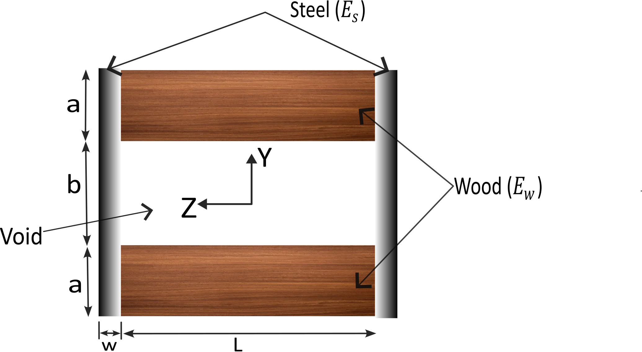
Solution: We first obtain bending stiffness of the cross-section. The cross-section being symmetrical, the neutral axis will be the mid horizontal line in the cross-section. The total bending stiffness of the cross-section will simply be \begin {align*} (EI)_{tot}= (EI)_{steel} + (EI)_{wood}=2 E_s \frac {1}{12}w\times (2a+b)^3 + E_w\frac {1}{12} L\left ((2a+b)^3-b^3)\right ). \end {align*}
(a) The curvature induced in the beam would then simply be \begin {align*} \kappa = M_z/(EI)_{tot}. \end {align*}
(b) Maximum bending stress in steel would be in its topmost/bottom-most fiber, i.e., \begin {align*} \sigma _s^{top} = E_s \kappa ~(a+b/2). \end {align*}
(c) Likewise, the maximum bending stress in the wood fiber will be in its topmost/bottom-most fiber, i.e., \begin {align*} \sigma _w^{top} = E_w \kappa ~(a+b/2). \end {align*}
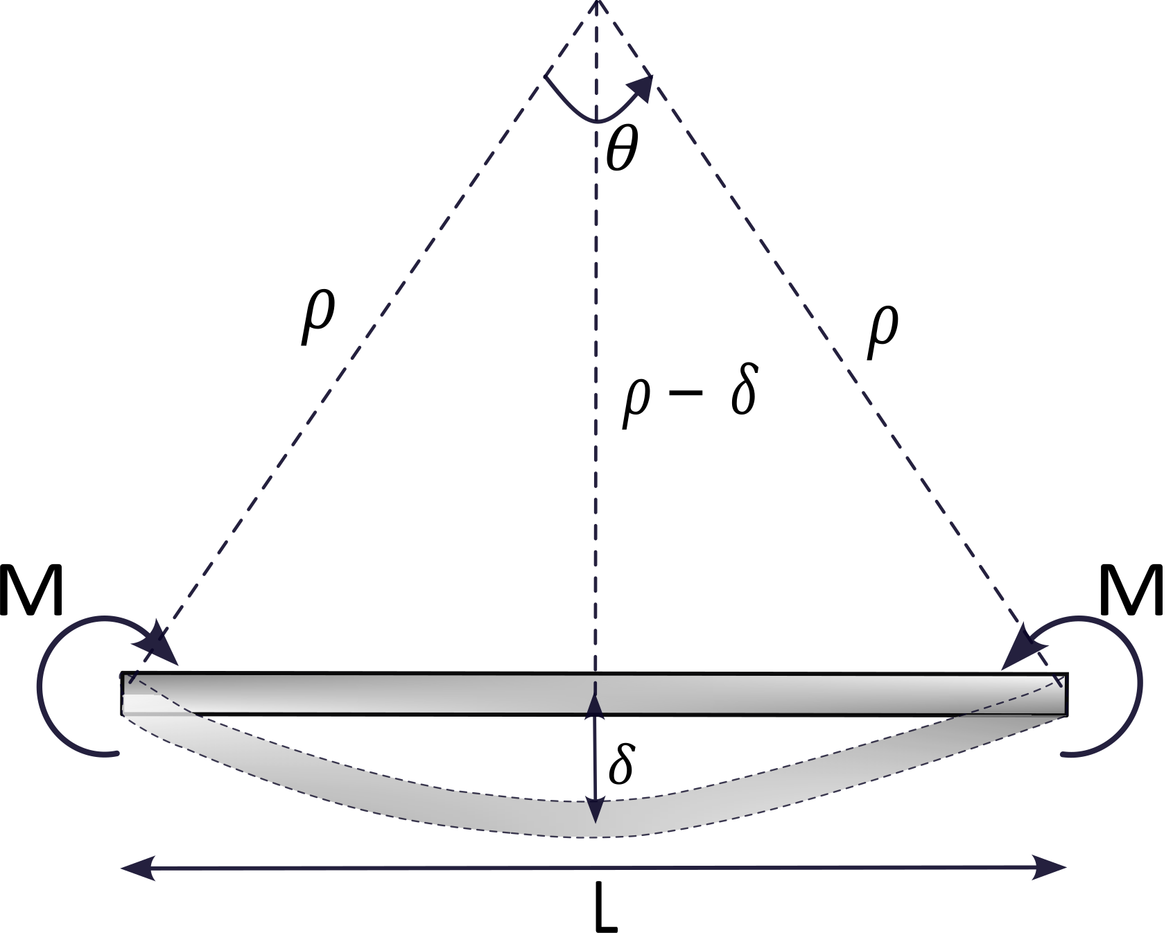
Solution: Note that the mid-point deflection of the bar is very small compared to its length. Therefore, in the above picture, we have drawn the ends of the deformed bar to also coincide with the ends of the undeformed bar. In reality, the deformed bar being curved, its two ends will be slightly inward compared to the undeformed bar. Neglecting this mismatch, we can write based on geometry that \begin {align*} \brc {\rho \;-\delta }^2\;+\;L^2/4\;=\;\rho ^2\Rightarrow \rho ^2\;-\;2\rho \delta +\delta ^2\;+\;L^2/4\;=\;\rho ^2 \quad \text {or}~\rho \;=\frac {L^2+4\delta ^2}{8\delta }. \end {align*}
Another way to obtain radius of curvature \(\rho \) is as follows. Let the angle subtended by the deformed beam at the center be \(\theta \). So, \(\rho \theta =L\). One can then write using trigonometry that \begin {align*} \rho \cos (\theta /2) = \rho -\delta &\Rightarrow \rho (1-\theta ^2/8) = \rho -\delta \quad \text {or}~ \rho = \frac {L^2}{8\delta }. \end {align*}
Here, we assumed \(\theta \) to be small. The couple required to generate this bending will be \begin {align*} &M\;=\;\dfrac {EI}{\rho }=\;\dfrac {E ~bh^3/12}{L^2/8\delta }=2/3\dfrac {Ebh^3\delta }{L^2}. \end {align*}
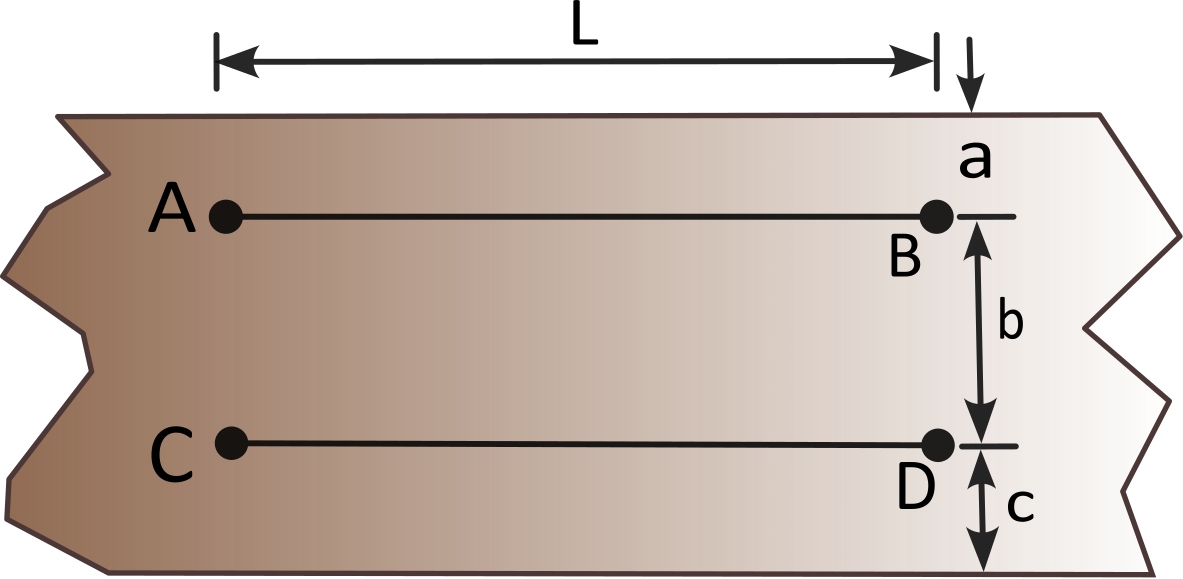
Solution: The picture above is that of a section of the beam along its length. The shape of the cross-section is not mentioned here. Accordingly, we can not assume that the neutral axis lies at the center. Let it lie at a distance \(x\) below the longitudinal fiber \(AB\). We know that \(\epsilon _{xx}=-\frac {y}{R}\). Hence \(\frac {y}{\epsilon _{xx}}\) must be a constant, i.e., \begin {align*} &\frac {x}{\epsilon _{AB}} = \frac {x-b}{\epsilon _{CD}} \Rightarrow \dfrac {x}{\frac {\delta _{AB}}{L}}\;=\;\dfrac {x-b}{-\frac {\delta _{CD}}{L}}~\text {or}~x\;=\;b/\left (1+\dfrac {\delta _{CD}}{\delta _{AB}}\right ). \end {align*}
We now obtain flexural/bending stress in the top fiber. We can write the following for the bending strain in the top fiber: \begin {align*} \frac {x}{\epsilon _{AB}} = \frac {x+a}{\epsilon _{top}}\Rightarrow \epsilon _{top} = \frac {x+a}{x}\epsilon _{AB}. \end {align*}
The bending stress in the top fiber will simply be \(E\epsilon _{top}\) since the longitudinal fibers are under uniaxial loading during pure bending. One can likewise obtain bending stress in the bottommost fiber.
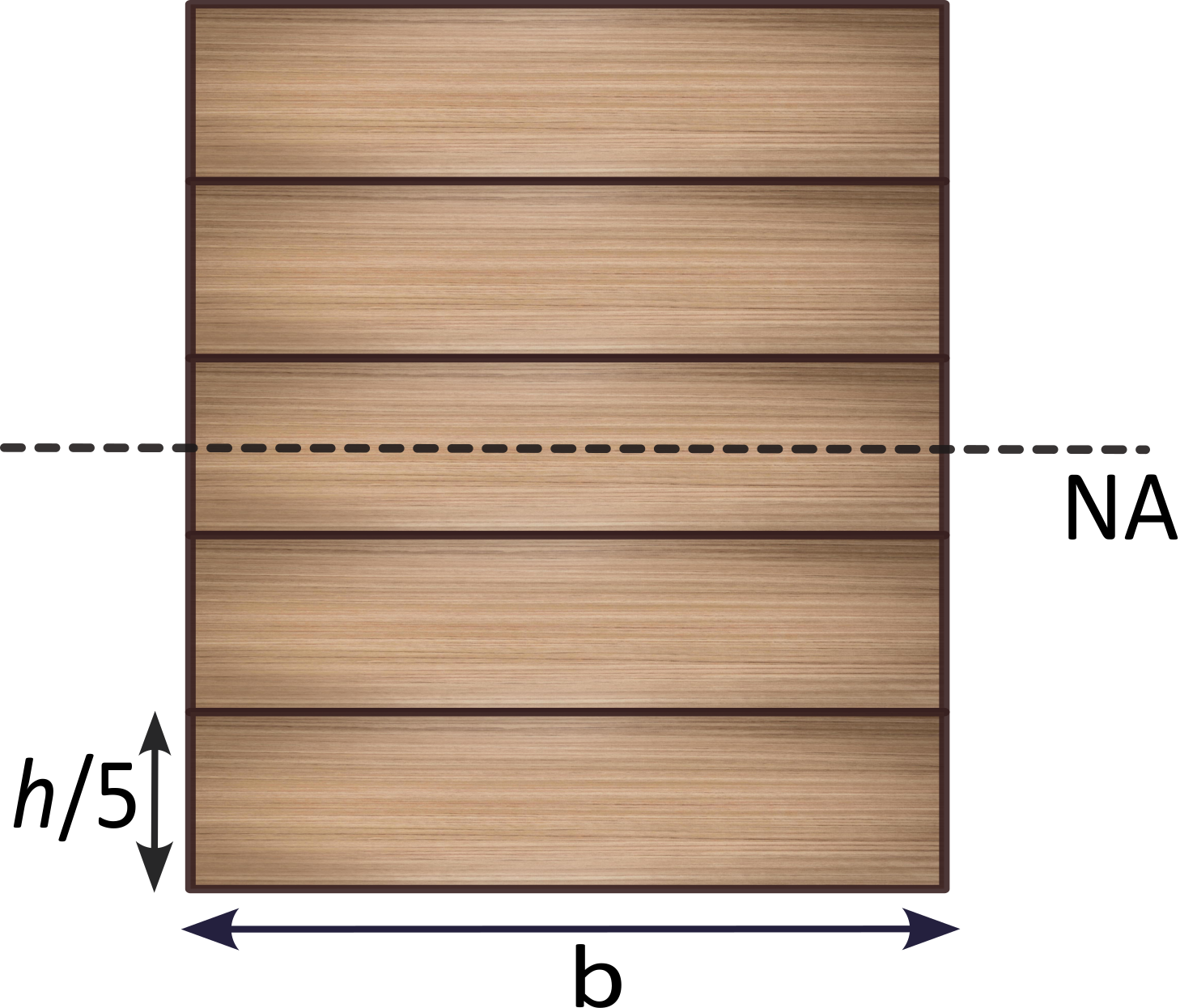
Determine the distributed load that such a simply supported beam can carry so that the allowable shear stress in the glue, wood and the allowable flexural stress in the wood are not crossed.
Solution: Let us assume that the uniformly-distributed load (UDL) is applied vertically downward. The application of UDL will lead to the generation of both bending moment and shear force at any cross-section. To find the maximum flexural and shear stress, we need to first obtain bending moment and shear stress distribution along the length of the beam. They are obtained through force and moment balance of an arbitrary portion of the beam as shown below (also illustrated in the figure below):
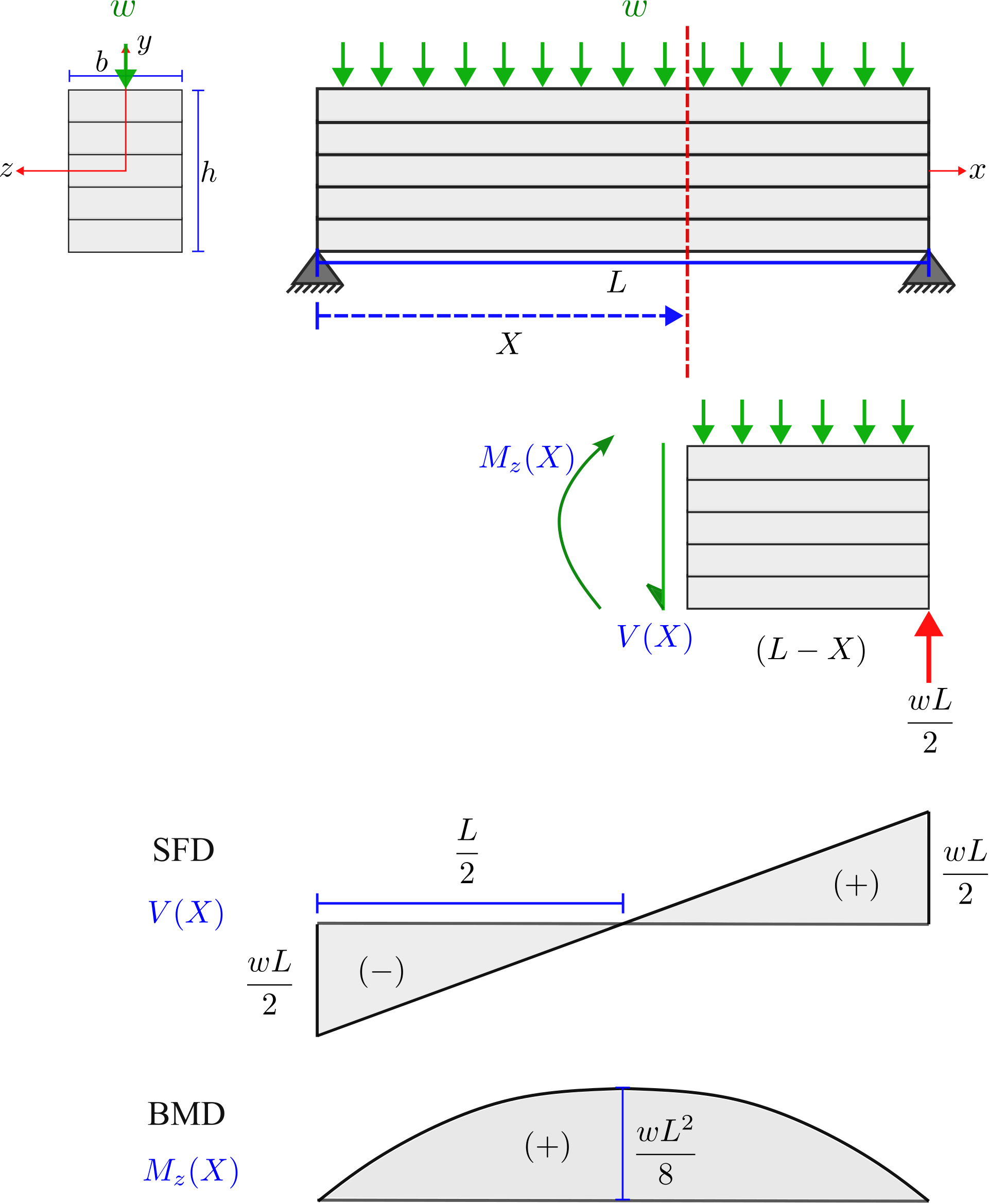
\begin {align*} \bullet \; &\uparrow + \sum F_y\;=\;0 \Rightarrow -V_x -w\brc {L\;-\;x}+\dfrac {wl}{2}=0 \Rightarrow V_x=-w\brc {\dfrac {L}{2}-x}. &\phantom {}\\ \bullet \;& \sum M_{\text {left end}} = 0 \text { (CCW sense +ve)}\\ & \Rightarrow -M_z\brc {x}+\dfrac {wl}{2}\brc {L-x}-\dfrac {w\brc {L-x}^2}{2}=0\Rightarrow M_z\brc {x}=\dfrac {wl}{2}\brc {L-x}-\dfrac {w\brc {L-x}^2}{2}. \end {align*}
Note that the bending moment is maximum at the center and vanishes at the two ends as is the case for
simply-supported beams. Due to symmetrical bending, the formulas for bending and shear stresses are
simpler:
\[\sigma _{xx}\;=\;\dfrac {M_z(x) \; y}{I_{zz}},\quad \tau _{yx}\;=\;\dfrac {V(x) \; Q(y)}{I_{zz} b}.\]
If the load were not applied along any of the principal axes, it would have resulted in unsymmetrical
bending.
Max bending stress \begin {align*} \sigma ^{wood}_{xx,\max }&=\max _{x,y} \cbk {\dfrac {M_z \brc {x}y }{I_{zz}}}=\dfrac {\max _{x} M_z\brc {x}}{I_{zz}} \max _{y} y=\dfrac {\brc {\dfrac {wL^2}{8} }\brc {\dfrac {h}{2}}}{\dfrac {1}{12} bh^3}=\;\dfrac {3wL^2}{4bh^2} \; \le \;\sigma _{xx,\text {tol}}^{\text {wood}} \;\; \ldots \;\; (1) \end {align*}
Max shear stress \begin {align*} \tau _{yx,\max }&=\max _{x,y} \dfrac {V\brc {x} \; Q\brc {y} }{I_{zz} \;b} = \dfrac {1}{I_{zz} b}\max _{x} V(x) \;\; \max _y Q(y)\\ \phantom {}&\\ Q\brc {y}&=\dfrac {b}{2}\brc {\dfrac {h^2}{4}\;-\;y^2} \Rightarrow \max _{y}Q\brc {y}=\;\dfrac {b}{2}\dfrac {h^2}{4}. \end {align*}
\[\therefore \;\tau ^{\text {wood}}_{yx,\max }=\dfrac {V\brc {x=L}}{I_{zz}}~\dfrac {Q\brc {y=0}}{b}\;=\;\dfrac {\dfrac {wL}{2}\brc {\dfrac {b}{2}\dfrac {h^2}{4}}}{\dfrac {1}{12}bh^3 \;b} = \frac {3 w L}{4 bh}\le \tau ^{\text {wood}}_{yx,\text {tol}} \;\; \ldots \;\; (2)\] The glue between two wooden planks resists shear stress generated between the planks. The shear stress at the level of the glue also should not exceed the maximum tolerable shear stress of glue. \[\therefore \;\tau ^{\text {glue}}_{yx,\max }\;=\;\dfrac {V\brc {x=L}}{I_{zz}}~\dfrac {Q\brc {y=\dfrac {h}{10}}}{b} =\dfrac {\dfrac {wL}{2}\brc {\dfrac {3bh^2}{25}}}{\dfrac {1}{12}bh^3 \;b} = \frac {18 w L}{25 bh}\;\leq \;\tau ^{glue}_{yx,\text {tol}} \;\; \ldots \;\; (3)\] From equations (1), (2), and (3), we would obtain three values of \(w\). The maximum allowed value of \(w\) would be the minimum of the values obtained from these three equations.
Solution: We will assume that the transverse load is acting along the principal axis of the beam resulting in symmetrical bending. Therefore, we can use the simpler formula \(\tau _{yx}\brc {x,y}\;=\;\dfrac {V Q(y)}{I_{zz} \; b\brc {y}} \). Note that unlike the beam with rectangular cross-section, the width of the I-beam is different in the flange and the web.
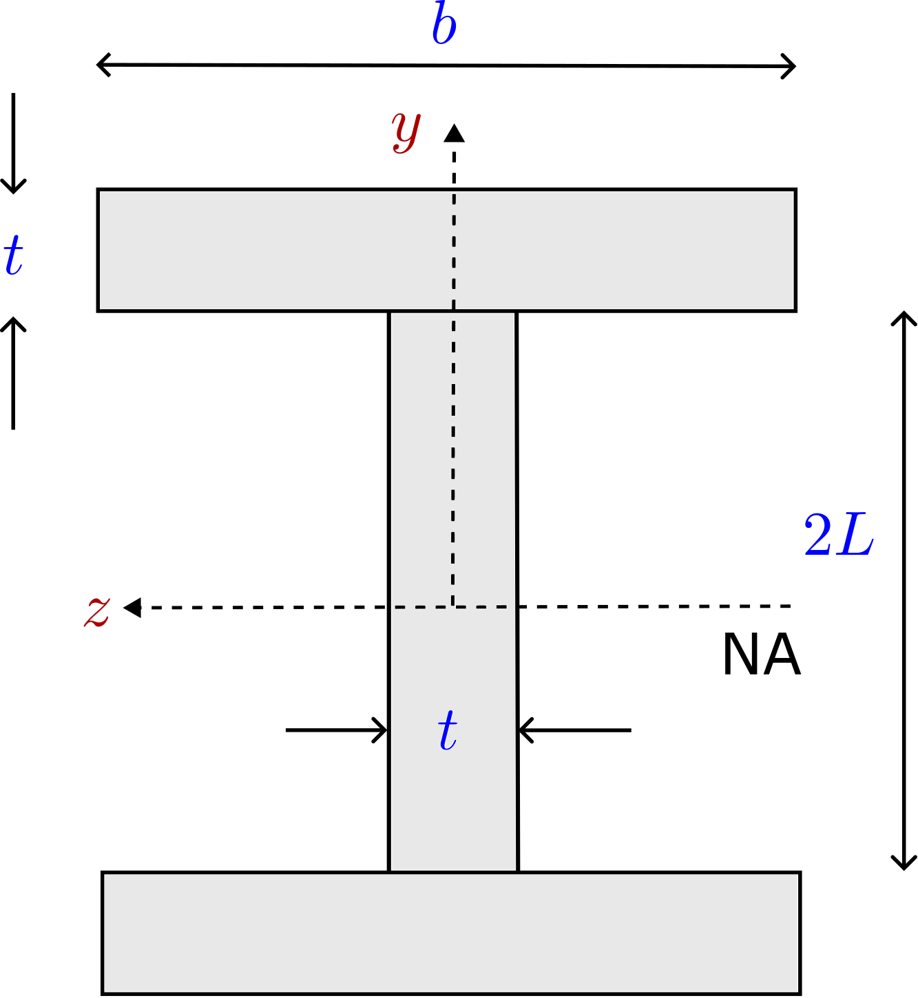
The shear force \(V\) is already given. Since we are looking at a section with fixed \(x\), only \(Q\brc {y}\) and \(b\brc {y}\) will change in the cross-section as \(y\) varies. Let’s first find the distribution of \(Q\brc {y}\). The neutral axis (NA) will be at the center and aligned with \(z\)-axis as shown in the figure.
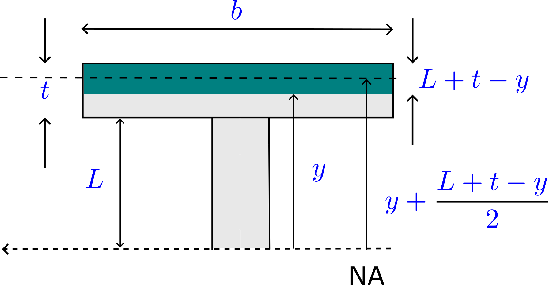
Calculation in the Flange region: \begin {align*} Q^f(y)\;&=\;b\brc { t\;+\;L\;-\;y}\times \sbk {y\;+\;\dfrac {t\;+\;L\;-y}{2} }\\ &=\dfrac {b}{2}\brc {t\;+\;L\;-y}\brc {t\;+\;L\;+\;y}=\dfrac {b}{2}\sbk {\brc {t\;+\;L}^2\;-\;y^2} \end {align*}
\begin {align*} \therefore \;\tau _{yx}\;&=\;\dfrac {V_x}{I_{zz}}\dfrac {\brc {b/2}}{b} \sbk {\brc {t\;+\;L}^2\;-\;y^2} \;\; \textcolor {blue}{(L \le y \le L+t)}\\ &=\;\dfrac {V_x}{2I_{zz}}\sbk {\brc {t\;+\;L}^2\;-\;y^2} \end {align*}
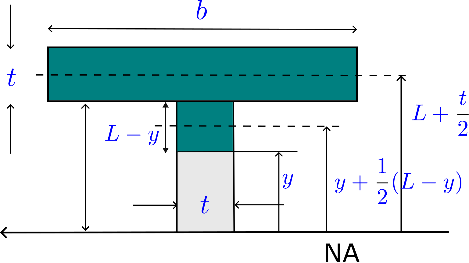
Calculation in the Web region: \begin {align*} Q^w(y) &= b \; t \times \brc {L+\dfrac {t}{2}} + t\brc {L-y}\times \dfrac {1}{2}\brc {L+y}= b \; t \brc {L+\dfrac {t}{2}} + \dfrac {t}{2} \brc {L^2 - y^2}\\ \therefore \;\tau _{yx}\;&=\;\dfrac {V_x}{I_{zz} \; t}\sbk {b \; t \brc {L+\dfrac {t}{2}} + \dfrac {t}{2} \brc {L^2 - y^2}} \end {align*}
\(I_{zz}\) for full I-beam \begin {align*} I^f_{zz} \text { (for flange) }&=\;\sbk {\dfrac {1}{12}bt^3\;+\;bt\brc {L\;+\;\dfrac {t}{2}}^2},\\ I^w_{zz} \text { (for web) }&=\;\dfrac {1}{12}\brc {2L}^3=\;\dfrac {8tL^3}{12},\\ I_{zz}\;&=\;2I^f_{zz}\;+\;I^w_{zz}. \end {align*}
(b) The variation of shear stress with respect to \(y\) is shown below:
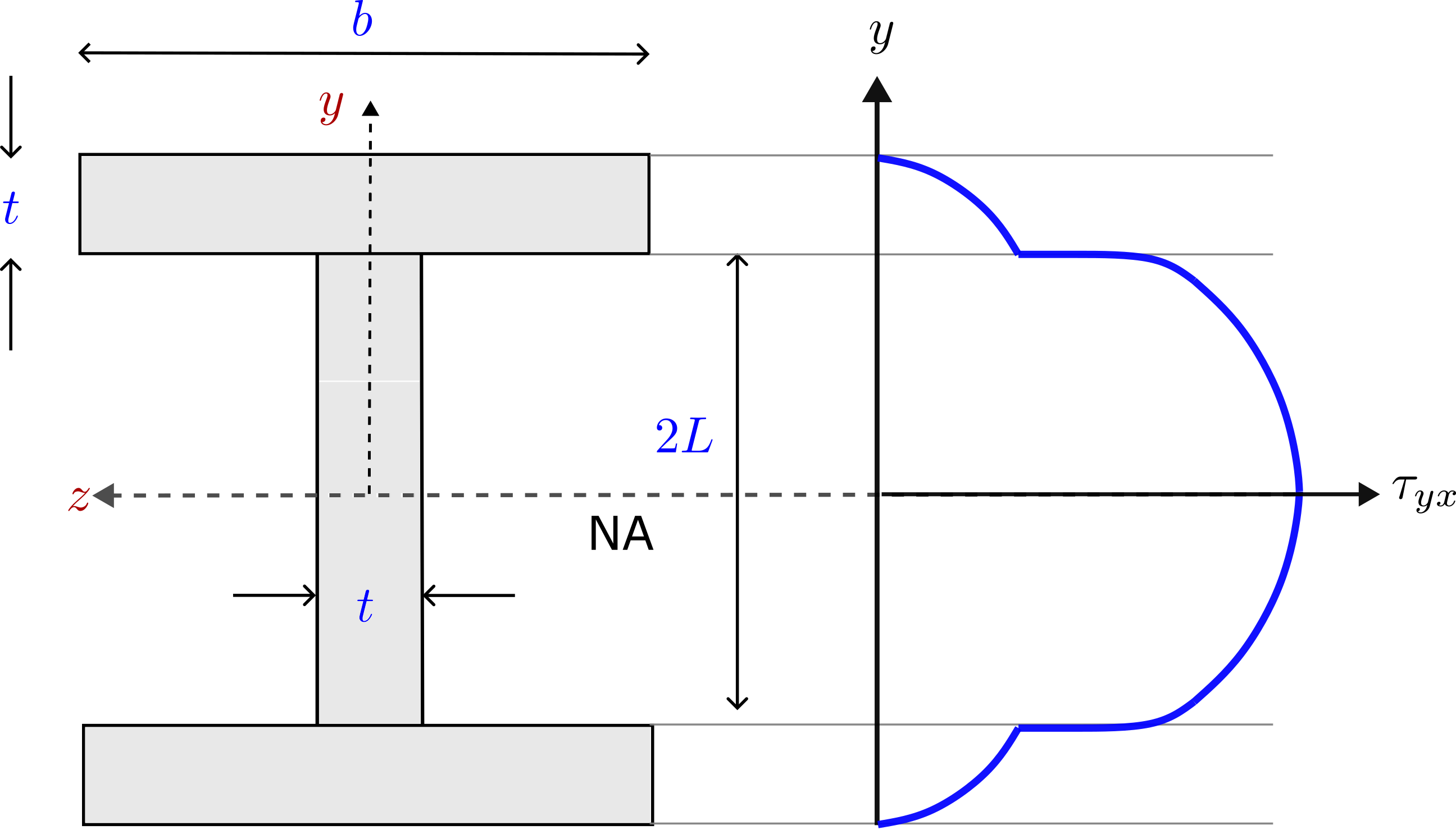
(c) Shear-stress is maximum at the NA
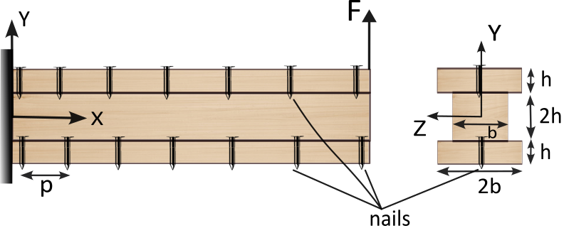
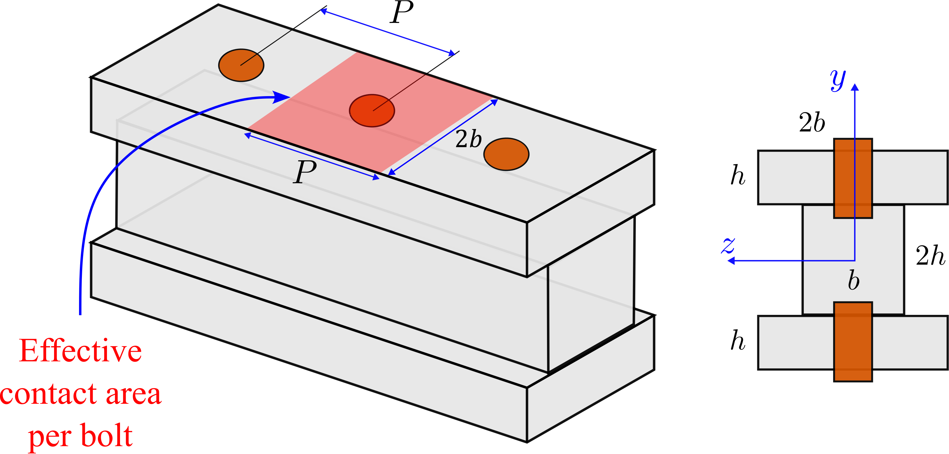
Solution: For the beam’s cross-section, its \(I_{zz}\) can be obtained using I-beam formula derived above leading to \(I_{zz}=10bh^3\). The effective area covered by each nail has a length equal to the spacing between nails. The total shear force between the two planks must be resisted by these nails. \begin {align*} \therefore \text {resistive shear force per nail}&=\;\tau _{yx}(\text {near interface in flange})\;\times \;\brc {2Pb}\\ &=\;\tau _{yx}(\text {near interface in web})\;\times \;\brc {Pb} \end {align*}
Notice that although shear stress exhibits a jump at the interface, the force experienced by each nail will not exhibit
such a jump. We need to now find shear stress at the interface of the two planks. Let’s first find \(Q(y=h)\) which will only have
a contribution from the full shaded region of flange as shown below.
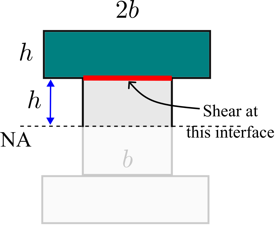
\begin {align*} \tau _{yx}(\text {near interface in web})\;&=\dfrac {V \brc {3bh^2}}{10bh^3\;\times \;b}=\;\dfrac {3V}{10bh}\\ \text {Resistive shear force/bolt}\;&=\;\dfrac {3V}{10bh}\;\times \;Pb=\dfrac {3VP}{10h}. \end {align*}
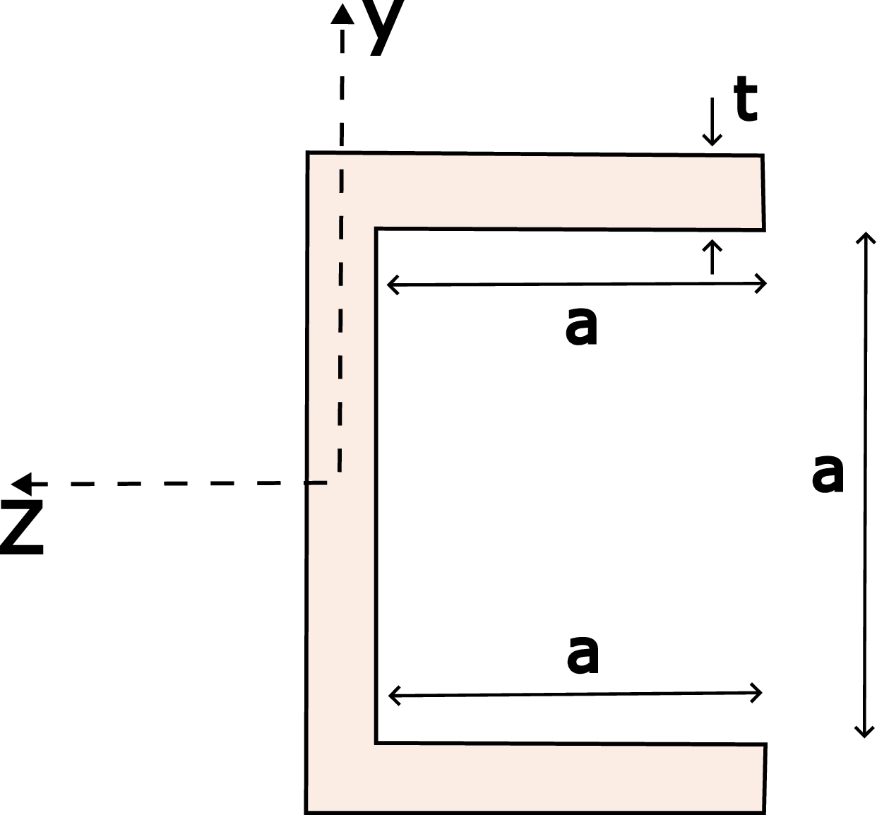
Solution: Since it is a thin tube (\(t<<a\)) and that the load is acting along principal axis, we can use the formula \[\tau _{sx}\;=\;-\dfrac {VQ_{sy}}{I_{zz} \;t}.\]
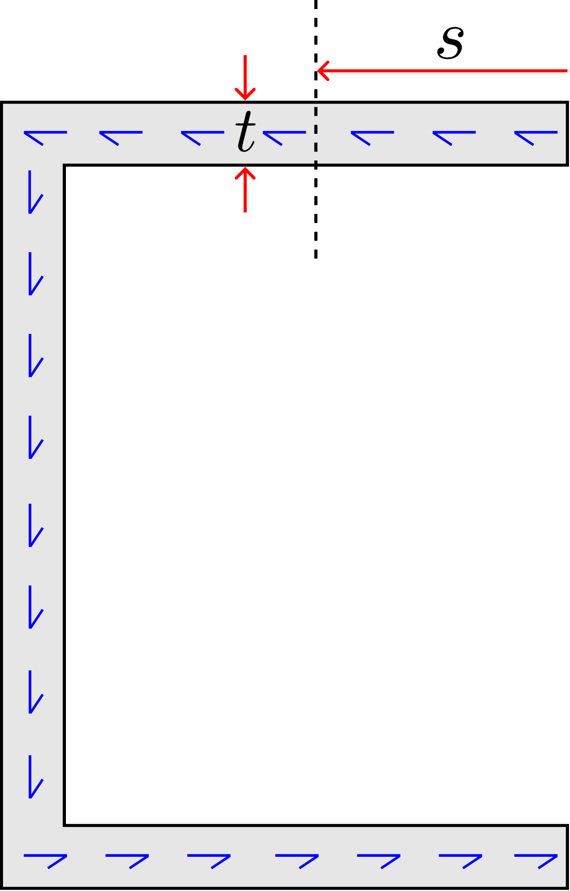
Shear stress lies along the cross section’s periphery as shown in the figure above! For the top horizontal flange portion (see subfigure (a) below), the shear stress is \begin {align*} \tau _{sx}\;=\;\dfrac {V\brc {\dfrac {a+t}{2}st} }{I_{zz}t}\;\approx \;\dfrac {Vas}{2I_{zz}}. \end {align*}
For the middle vertical web portion (see subfigure (b) below), the shear stress is \begin {align*} \tau _{sx}\;&=\;\dfrac {V\brc {\dfrac {a}{2}at\;+\;\sbk {s\;+\;\brc {\dfrac {a}{2}\;-\;s }/2 }\brc {\dfrac {a}{2}\;-\;s}t } }{I_{zz}t}=\;\dfrac {V\brc {\dfrac {a^2}{2}\;+\;\dfrac {1}{2}\brc {\dfrac {a^2}{4}\;-\;s^2}} }{I_{zz}}. \end {align*}
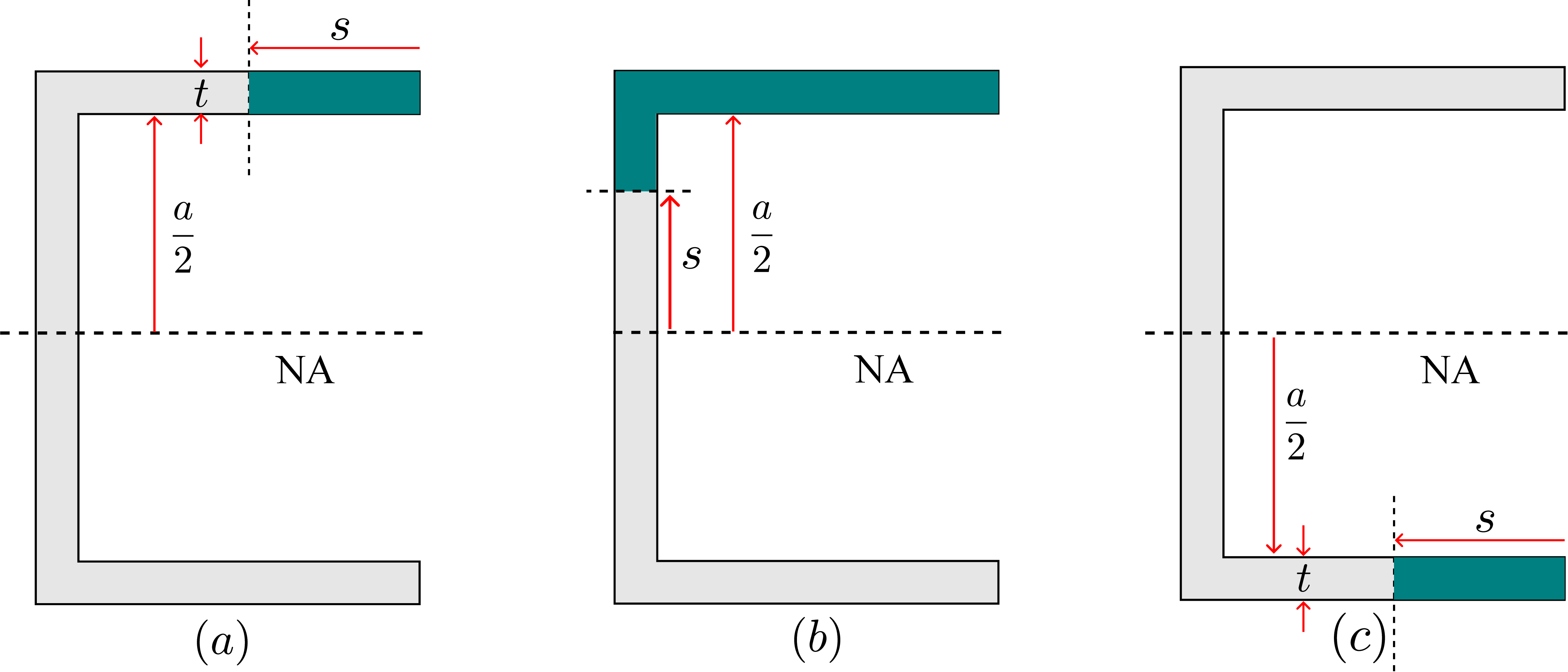
For the bottom horizontal flange portion (see subfigure (c) above), the shear stress is \begin {align*} \tau _{sx}\;&=\;\dfrac {VQ}{I_{zz}t}=\;\dfrac {V\brc {-\dfrac {a}{2}st }}{I_{zz}t}=\;-\dfrac {Vas}{2I_{zz}}. \end {align*}
The moment of area can be calculated separately for each of the three parts (top, middle and lower) about their own centroidal axis and then shifted to the NA as shown below: \begin {align*} I_{zz}\;=\;I_{zz}\brc {1}\times 2\;+\;I_{zz}\brc {2}=\;\sbk {\dfrac {1}{12}at^3\;+at\brc {\dfrac {a}{2}}^2 }\times 2\;+\;\dfrac {1}{12}a^3t=\dfrac {1}{6}at^3\;+\;a^3t\dfrac {7}{12}. \end {align*}
The shear center is the location of the point in/outside the cross-section at which a load applied parallel to the plane of the section will produce no twisting. To obtain shear center, first obtain torque due to shear stress distribution about origin.
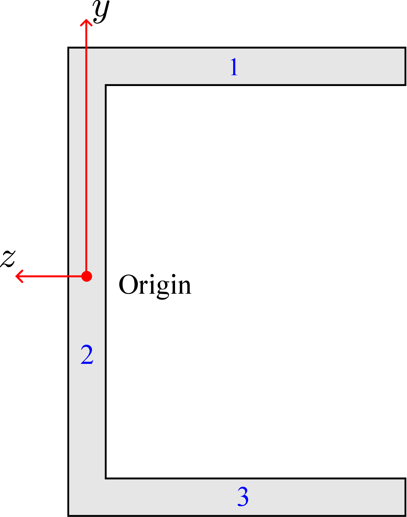
\begin {align*} T\;=\; T_1 +T_2 + T_3&=\;T_1\times 2 + T_2~\text {(regions 1 and 3 contribute same torque)}\\ &=\sbk {\dfrac {Vat}{2I_{zz}}\int ^a_0 sds \times \dfrac {a}{2} }\times 2\;+\;0 =\;\dfrac { Va^4t}{8I_{zz}}\times 2\;=\;\dfrac {Va^3}{4\brc {t^2/6\;+\;7/12a^2 }}. \end {align*}
Note that torque due to region 2 is zero because shear stress there passes through origin! Location of shear center \(=\;\dfrac {a^3}{4 \brc {t^2/6\;+\;7/12a^2 }}\) along \(-z\)-axis.
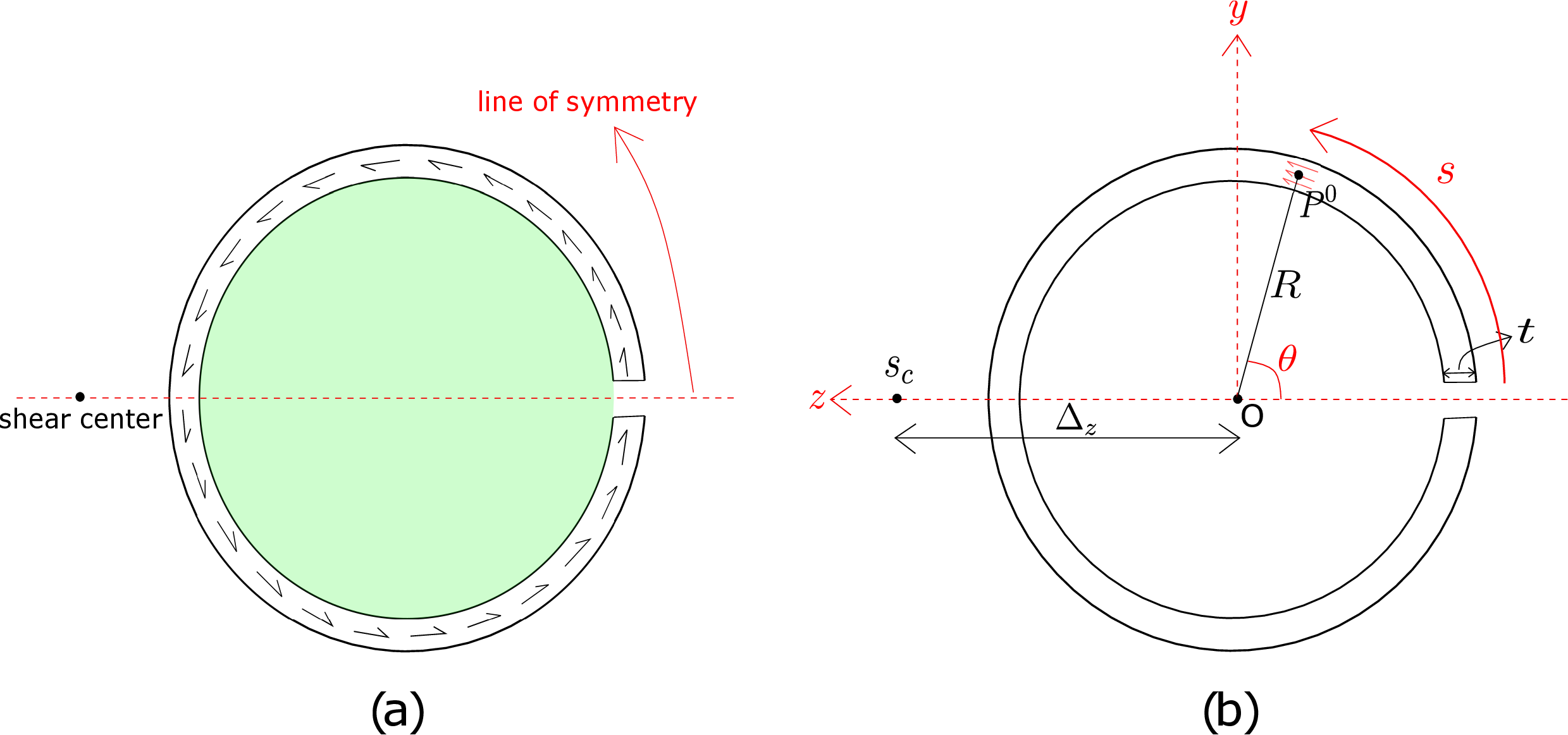
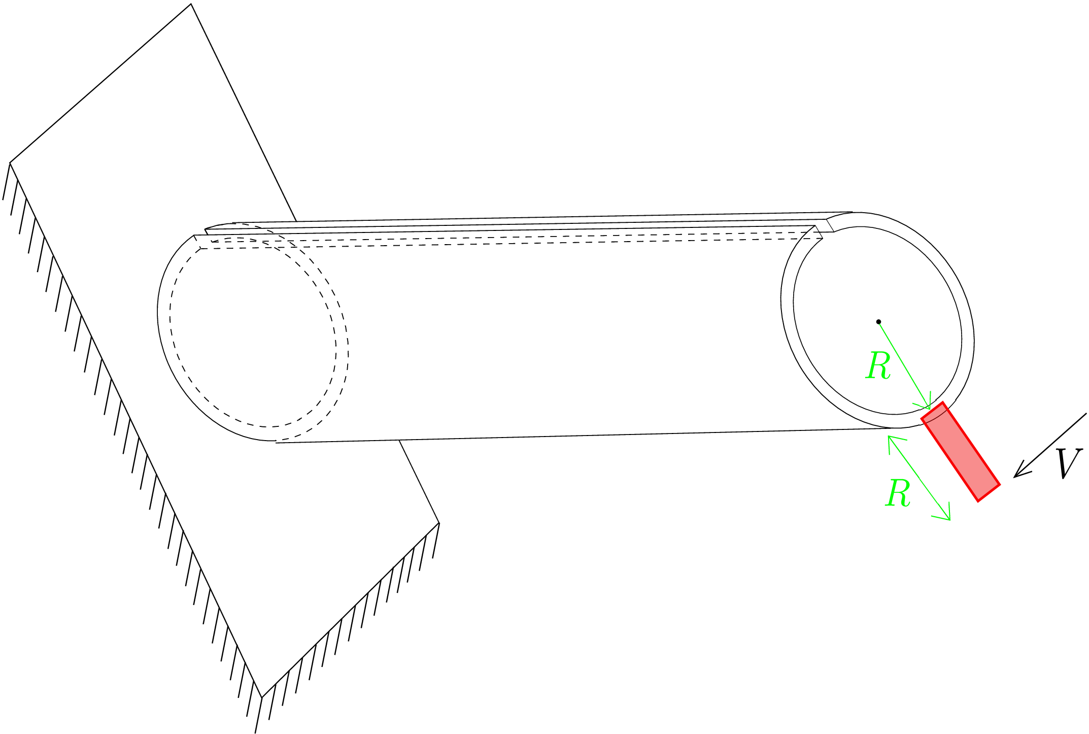
Solution: For such a cross-section, we have only one line of symmetry due to the presence of a cut. Thus, the shear
center lies on this line of symmetry. As the cross section is thin and open, shear stress also flows from one
end to the other. If we find torque about any point in the green region (see Figure 8.27a), the torque
due to all the shear stresses contribute in the same direction and hence does not vanish. Thus, the
shear center must lie outside this green region. Let us try to find the exact location of shear center.
Suppose that the mean radius of the annulus is \(R\) and thickness is \(t\). As the shear center has to lie on the line of
symmetry, \(\Delta _y=0\). Notice that even though there is an infinitesimal cut in the cross-section, any pair of perpendicular lines
will still form the cross-section’s principal axes, in particular, the (\(y-z\)) axis also form a principal axes pair. We can thus
use formula \eqref{8_z_coord} to obtain \(\Delta _z\) which can be alternatively written in terms of \(\theta \) coordinate as follows:
We need to now find \(Q_y^{\theta }\) for the region \([0,\theta ]\) (see Figure 8.27b) which has also been drawn separately in Figure 8.28.
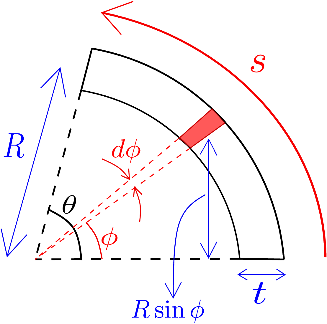
Let us consider a tiny strip shown in red in Figure 8.28 which subtends an angle \(d\phi \) at the center. The \(y\)-coordinate of the centroid of this tiny strip is \(R\sin \phi \) and its area is \(tRd\phi \). Thus, for this tiny strip, we can write:
We can now find \(Q_y^{\theta }\) by integrating over such tiny strips, i.e.
Let us now find \(I_{zz}\) for the cross-section about its centroid O. As the cut is really thin, the annulus is approximately complete. So, to calculate \(I_{xx}\), \(I_{yy}\) and \(I_{zz}\), we can forget about the thin cut. We thus have \begin {equation} \label {8_I_zz} I_{zz}=I_{yy}=1/2~I_{xx}=1/2 ~R^2~(2\pi R~t)=\pi R^3~t. \end {equation} Finally substituting equations \eqref{8_Q_y} and \eqref{8_I_zz} into equation \eqref{8_z_shear}, we obtain \begin {equation} \Delta _z=\frac {R}{\pi }\int _{0}^{2\pi }(1-cos\theta )~d\theta =2R. \end {equation} The shear center thus does not lie on the cross-section. As discussed earlier, if we want to apply shear force on beams having such cross-sections so that the beam does not twist, we must apply shear force so that its line of action passes through shear center. For the present cross-section, we need to create an extension of it (e.g., by a thin rod as shown in red in Figure 8.29) and apply shear force there so that the beam indeed does not twist.
∗A moment applied along the beam’s axis is called torque whereas a moment applied transverse to the beam’s axis is called bending moment.
†The two shear stress components turn out to be zero in case of pure bending.
‡For a straight beam, the radius of curvature is \(\infty \).
§If the cross-section were closed and say we choose \(s=0\) at some point, then we won’t be able to say for sure if \(\tau _{sx}\) is vanishing on \(s\)=0 plane - it would become an unknown in the derivation.