As of now, we have worked with Cartesian coordinate system - be it about representing stress and strain tensors or deriving stress equilibrium equations or solving deformation problems. However, there are many deformation problems where working with cylindrical coordinate system turns out to be handy such as in studying axisymmetric deformation of cylindrical bodies.∗ It is therefore of importance to obtain stress and strain matrices as well as stress equilibrium equations in cylindrical coordinate system. We achieve this task in this chapter. We begin with first discussing the cylindrical coordinate itself and then derive stress equilibrium equations in this coordinate system. We further obtain expressions of components of strain matrix in cylindrical coordinate system. Finally, we solve axisymmetric problems such as extension, torsion and inflation of cylinders, rotating shaft problem, shrunk-fit problem etc. using cylindrical coordinate system.
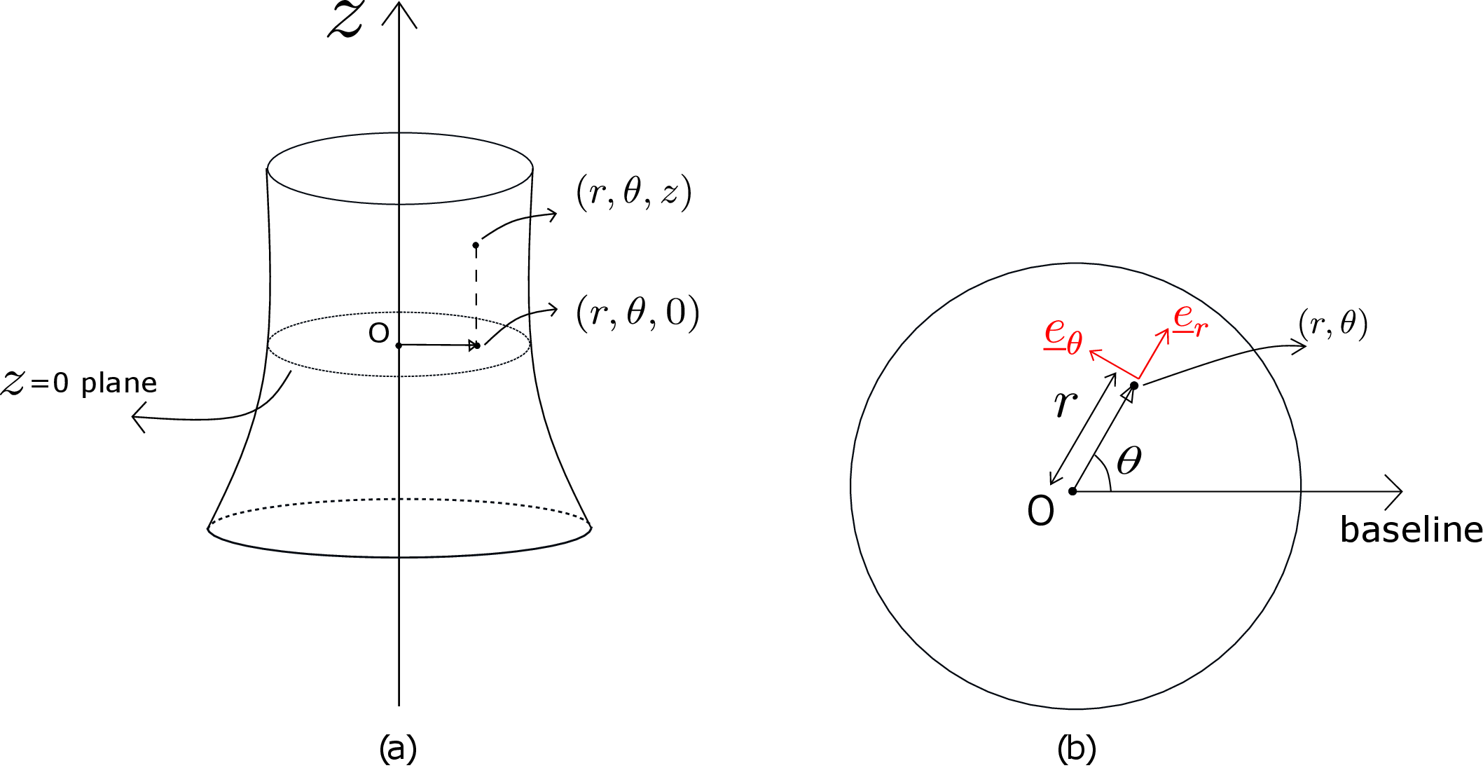
Figure 7.1a shows a generalized cylinder whose radius may change along the axis of the cylinder.
The axis of the cylinder coincides with \(z\) axis. Any general point of the cylinder will have coordinates \((r,\theta ,z)\). The position vector of this point is \(r\underline {e}_r+z\underline {e}_z\) where the \(\theta \)-dependence is hidden in the basis vector \(\underline {e}_r\). If we project this point on \(z=0\) plane, we get to \((r,\theta ,0)\) as shown in Figure 7.1a. We have drawn the \(z=0\) plane in Figure 7.1b. There is a baseline or a reference line relative to which angle \(\theta \) is measured. The length of the line joining the center and the projected point is \(r\) while the angle that it makes from the baseline is \(\theta \). Two of the basis vectors lie in this plane: \(\underline {e}_r\) points radially outward from the center while \(\underline {e}_\theta \) points in the direction of increasing \(\theta \) and is perpendicular to \(\underline {e}_r\). The third basis vector \(\underline {e}_z\) lies along the axis of the cylinder. Thus, the basis vectors for a cylindrical coordinate system are \((\underline {e}_r,\underline {e}_\theta ,\underline {e}_z)\) whereas in Cartesian coordinate system, the basis vectors are \((\underline {e}_1,\underline {e}_2,\underline {e}_3)\). Although both the sets of basis vectors are orthonormal, there is a big difference in their properties: the basis vectors of Cartesian coordinate system are fixed in direction and do not change from one point to the other but in cylindrical coordinate system, two of the basis vectors \((\underline {e}_r,\underline {e}_\theta )\) change when \(\theta \)-coordinate of a point changes. This has been illustrated in Figure 7.2a where the basis vectors at the two points are differently oriented although only the \(\theta \)-coordinate of the two points is different.
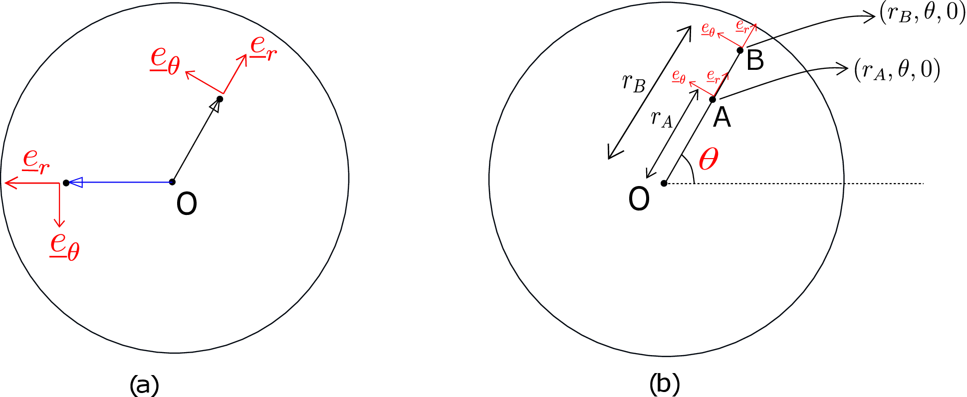
The third basis vector \(\underline {e}_z\) remains fixed at every point though. It may be emphasized here that \(\underline {e}_r\) and \(\underline {e}_\theta \) change
only when the \(\theta \)-coordinate changes. If only the radial coordinate or/and z-coordinate of a point is changed,
the basis vectors do not change (see Figure 7.2b).
We now show how to obtain \(\dfrac {\partial \underline {e}_r}{\partial \theta }\) and \(\dfrac {\partial \underline {e}_\theta }{\partial \theta }\). We again draw \(z=0\) plane as shown in Figure 7.3a.
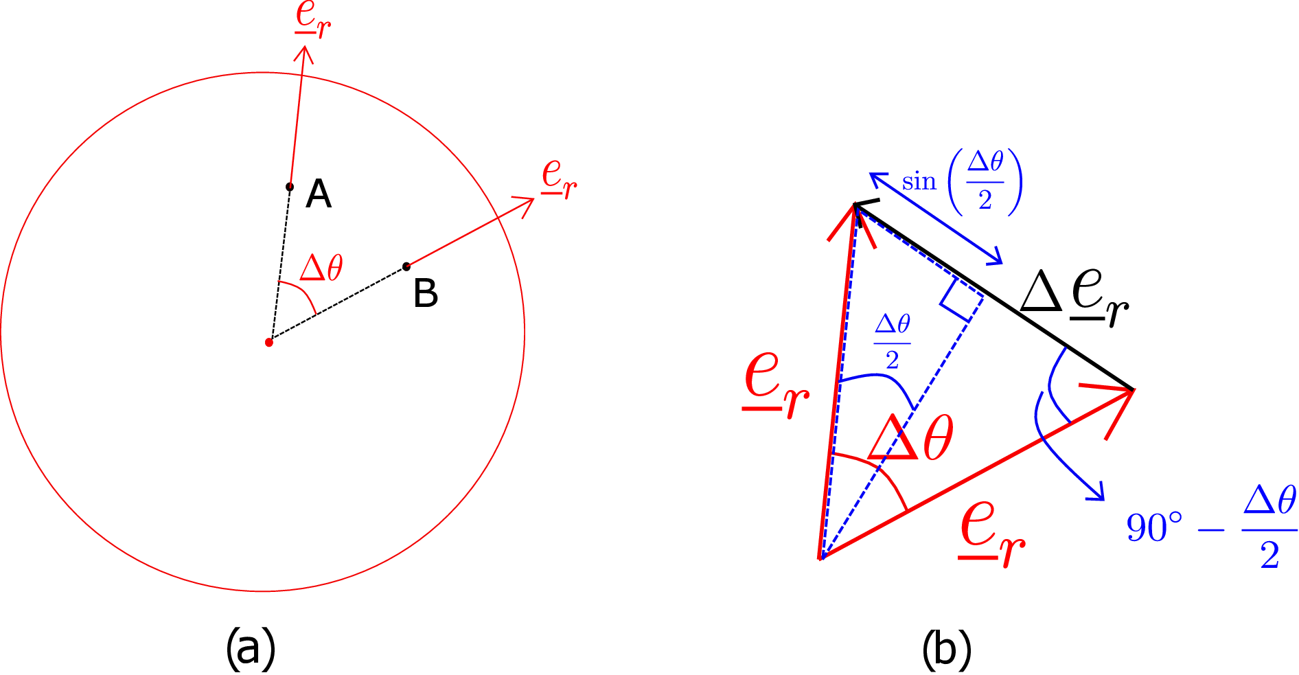
The \(\theta \)-coordinates of the two points A and B differ by \(\Delta \theta \). Using the definition of differentiation, we can write \begin {equation} \label {7_fundamental_calculus} \frac {\partial \underline {e}_r}{\partial \theta }=\lim _{\Delta \theta \to 0}\frac {\underline {e}_r(\theta +\Delta \theta )-\underline {e}_r(\theta )}{\Delta \theta }. \end {equation} To obtain it geometrically, we parallelly transport the two radial vectors such that they start from a common point as shown in Figure 7.3b. The angle between the two radial vectors is still \(\Delta \theta \). The numerator in equation \eqref{7_fundamental_calculus} will thus equal the third side of the triangle in Figure 7.3b which is also denoted by \(\Delta \underline {e}_r\) there. The magnitude of the two sides representing the basis vectors has magnitude 1 as they are unit vectors. We then draw an angle bisector to the angle \(\Delta \theta \). As the original triangle is an isosceles triangle, the angle bisector is also the perpendicular bisector to the base. Let us then consider any one of the two right triangles: the magnitude of its base equals \(\sin (\frac {\Delta \theta }{2})\). So, the total magnitude of \(\Delta \underline {e}_r\) will be \(2\sin (\frac {\Delta \theta }{2})\). Let us denote the direction of this vector by \(\underline {e}\). Substituting these results in equation \eqref{7_fundamental_calculus}, we get \begin {equation} \label {derivative_of_basis_r} \frac {\partial \underline {e}_r}{\partial \theta }=\lim _{\Delta \theta \to 0}\frac {2\sin (\frac {\Delta \theta }{2})}{\Delta \theta }\underline {e} \end {equation} The direction \(\underline {e}\) makes an angle of \(90^\circ -\frac {\Delta \theta }{2}\) with \(\underline {e}_r\) as shown in Figure 7.3b. In the limit of \(\Delta \theta \to 0\), this angle becomes \(90^\circ \). Thus, in this limit, \(\Delta \underline {e}_r\) points along \(\underline {e}_\theta \). Also, the magnitude term in equation \eqref{derivative_of_basis_r} becomes 1 (\(\because \lim _{x\to 0}\frac {\sin x}{x}=1\)). Thus, we finally have \begin {equation} \frac {\partial \underline {e}_r}{\partial \theta }=\underline {e}_\theta . \end {equation} A similar derivation shows that \begin {equation} \frac {\partial \underline {e}_\theta }{\partial \theta }=-\underline {e}_r. \end {equation}
In Cartesian coordinate system, we worked with cuboid elements with their face normals directed along the three coordinate axes. In cylindrical coordinate system similarly, we will work with cylindrical elements with their face normals parallel to \(\underline {e}_r\), \(\underline {e}_\theta \) and \(\underline {e}_z\). A small cylindrical element within a generalized cylinder and its zoomed view is shown in Figure 7.4.
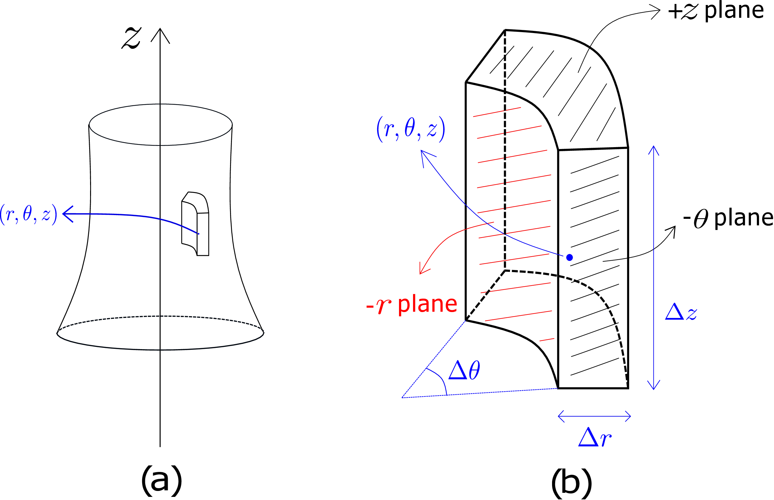
The top face has its normal along \(z\) axis. Thus, the top face is \(+z\) plane and the bottom face is \(-z\) plane. The front face shown has its normal along \(-\underline {e}_\theta \) direction. Thus, this is \(-\theta \) plane and the plane opposite to it is \(+\theta \) plane. Finally, the concave curved face has its plane normal along \(-\underline {e}_r\) direction and can be imagined to become flat in the limit of the cylindrical element becoming infinitesimally small. Likewise, the convex curved face is \(+r\) plane.
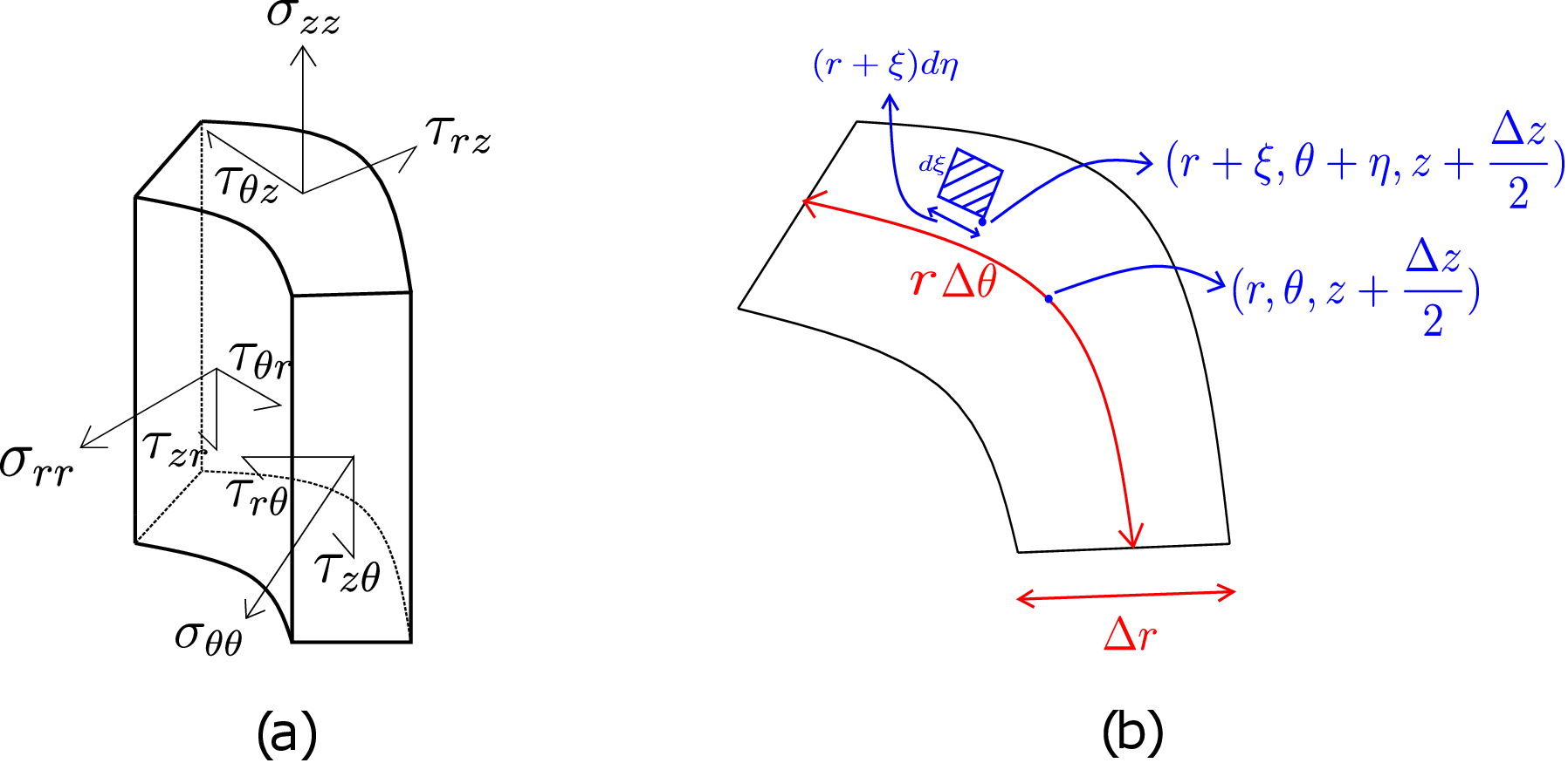
For linear momentum balance, we need to sum the forces acting on the cylindrical element due to tractions and body force and equate it to the cylindrical element’s rate of change of linear momentum. Let us begin with considering each of the faces separately, obtain total force on them and eventually add all of them. In Figure 7.5a, we have shown the traction components (resolved along the three basis vectors) acting on each of these faces from the remaining part of the body.
On \(+z\) plane, the traction vector \(\underline {t}^{+z}\) is given by \begin {equation} \underline {t}^{+z}=\sigma _{zz}\underline {e}_z+\tau _{rz}\underline {e}_r+\tau _{\theta z}\underline {e}_\theta . \end {equation} The total force due to this traction can be obtained by integrating it over \(+z\) plane which we have drawn separately in Figure 7.5b. The difference between the outer and inner radii of this face is \(\Delta r\) and the total angle subtended by the face at the center is \(\Delta \theta \). The center of the cylindrical element shown in Figure 7.4 and likewise Figure 7.5a has coordinates \((r,\theta ,z)\). Thus, the coordinates of a general point on its top surface is denoted by \((r+\xi ,\theta +\eta ,z+\frac {\Delta z}{2})\) (\(r\) and \(\theta \) coordinates vary while \(z\) coordinate remains fixed). We then consider an infinitesimal area element on this face. The length of this area element in the radial direction is \(d\xi \) and its width in \(\theta \)-direction is \(r\)-coordinate multiplied with \(d\eta \). Thus, the area of the infinitesimal element is
Hence, the total force on \(+z\) plane is
For \(-z\) plane, all the traction components act along negative basis directions but an arbitrary point on \(-z\) plane will have coordinates \((r+\xi ,\theta +\eta ,z-\frac {\Delta z}{2})\). Thus, the total force on \(-z\) plane will be
As the stress components are varying in the domain of integration, we can use Taylor’s expansion about the center of the cylindrical element, i.e., at \((r,\theta ,z)\). In equation \eqref{7_F_plus_z_before_Taylor}, e..g, we need to Taylor expand both stress components as well as basis vectors. Ignoring higher order terms, we get
As \(\underline {e}_r\) and \(\underline {e}_\theta \) change only with \(\theta \), their partial derivatives with respect to \(r\) and \(z\) are not present in the above expression. Upon further plugging the derivatives of basis vectors into above equation, we get
Let us now consider the first set of terms, i.e., \begin {equation} \label {7_zface} \iint \,\bigg [\sigma _{zz}+\frac {\partial \sigma _{zz}}{\partial r}\xi +\frac {\partial \sigma _{zz}}{\partial \theta }\eta +\frac {\partial \sigma _{zz}}{\partial z}\frac {\Delta z}{2}\bigg ]\underline {e}_z dA. \end {equation} In the first term here, \(\sigma _{zz}\) is is evaluated at the center of the cylindrical element and hence can be taken out of the integral. The integral of \(dA\) then gives us \(A_z\): the area of \(+z\) face.† Similar logic applies to the last term here. Considering the second term, the integration of \(\xi dA\) will give us \(A_z\) times \(r_{\text {centroid}}\) of \(+z\) face. As we are measuring \(\xi \) from the centroid itself, \(r_{\text {centroid}}\) becomes zero. Likewise, the integration of \(\eta dA\) in the third term will be zero. Thus, equation \eqref{7_zface} becomes
Here \(\frac {\Delta V}{2}\) denotes half the volume of the cylindrical element. Now, consider the second set of terms in equation \eqref{7_F_z_sets_of_terms}: \begin {equation} \iint \bigg [\tau _{rz}+\frac {\partial \tau _{rz}}{\partial r}\xi +\frac {\partial \tau _{rz}}{\partial \theta }\eta +\frac {\partial \tau _{rz}}{\partial z}\frac {\Delta z}{2}\bigg ]\bigg (\underline {e}_r+\eta \underline {e}_\theta \bigg )dA. \end {equation} The integration of the big bracket multiplied with \(\underline {e}_r\) will give us \(\bigg [\tau _{rz}A_z+\dfrac {\partial \tau _{rz}}{\partial z}\dfrac {\Delta V}{2}\bigg ]\underline {e}_r\) by a similar analysis as used for the first set of terms. Let us now look at multiplication of the big bracket with the second term. The terms \(\tau _{rz}\), its partial derivatives and \(\underline {e}_\theta \) are constant in the domain of integration as they are evaluated at the center of the cylindrical element. Thus, the first term will be \(\tau _{rz}\underline {e}_\theta \iint \eta dA\) which will be zero again. For the second term, we will get
The third term is \(\dfrac {\partial \tau _{rz}}{\partial \theta }\underline {e}_\theta \iint \eta ^2 dA\). When we work this out, we will get something that is of the order higher than the volume of the cylindrical element, i.e., o(\(\Delta V\)). This is because both \(\eta ^2\) and \(dA\) terms have dimension squared of the length. Thus the integration will be fourth power in length. The last term \(\dfrac {\partial \tau _{rz}}{\partial z}\underline {e}_\theta \dfrac {\Delta z}{2}\iint \eta dA\) will also become zero. Thus, the second set of terms in \eqref{7_F_z_sets_of_terms} finally gives us \begin {equation} \iint \bigg [\tau _{rz}+\frac {\partial \tau _{rz}}{\partial r}\xi +\frac {\partial \tau _{rz}}{\partial \theta }\eta +\frac {\partial \tau _{rz}}{\partial z}\frac {\Delta z}{2}\bigg ]\bigg (\underline {e}_r+\eta \underline {e}_\theta \bigg )dA=\bigg [\tau _{rz}A_z+\frac {\partial \tau _{rz}}{\partial z}\frac {\Delta V}{2}\bigg ]\underline {e}_r+o(\Delta V) \end {equation} The last set of terms in \eqref{7_F_z_sets_of_terms} can be similarly integrated to yield \begin {equation} \iint \bigg [\tau _{\theta z}+\frac {\partial \tau _{\theta z}}{\partial r}\xi +\frac {\partial \tau _{\theta z}}{\partial \theta }\eta +\frac {\partial \tau _{\theta z}}{\partial z}\frac {\Delta z}{2}\bigg ]\bigg (\underline {e}_\theta -\eta \underline {e}_r\bigg )dA=\bigg [\tau _{\theta z}A_z+\frac {\partial \tau _{\theta z}}{\partial z}\frac {\Delta V}{2}\bigg ]\underline {e}_\theta +o(\Delta V). \end {equation} The total force on \(+z\) plane will thus be \begin {equation} \label {7_Final_F_plus_z} \underline {F}^{+z}=\bigg (\sigma _{zz}A_z+\frac {\partial \sigma _{zz}}{\partial z}\frac {\Delta V}{2}\bigg )\underline {e}_z+\bigg (\tau _{rz}A_z+\frac {\partial \tau _{rz}}{\partial z}\frac {\Delta V}{2}\bigg )\underline {e}_r+\bigg (\tau _{\theta z}A_z+\frac {\partial \tau _{\theta z}}{\partial z}\frac {\Delta V}{2}\bigg )\underline {e}_\theta +o(\Delta V). \end {equation} We can also find the force on \(-z\) plane in the same way. If we compare equations \eqref{7_F_plus_z_before_Taylor} and \eqref{F_minus_z_before_Taylor}, we find that we have an overall negative sign for the \(-z\) plane and also the stress components are to be evaluated at \(z-\dfrac {\Delta z}{2}\) instead of \(z+\dfrac {\Delta z}{2}\). So, whenever we will have a term of the form \(\dfrac {\partial }{\partial z}\), it will be multiplied with \(\dfrac {-\Delta z}{2}\). The overall negative sign will then make such terms positive while the other terms will become negative. Thus, we will get \begin {equation} \label {7_Final_F_minus_z} \underline {F}^{-z}=\bigg (-\sigma _{zz}A_z+\frac {\partial \sigma _{zz}}{\partial z}\frac {\Delta V}{2}\bigg )\underline {e}_z+\bigg (-\tau _{rz}A_z+\frac {\partial \tau _{rz}}{\partial z}\frac {\Delta V}{2}\bigg )\underline {e}_r+\bigg (-\tau _{\theta z}A_z+\frac {\partial \tau _{\theta z}}{\partial z}\frac {\Delta V}{2}\bigg )\underline {e}_\theta +o(\Delta V). \end {equation} Upon adding equations \eqref{7_Final_F_plus_z} and \eqref{7_Final_F_minus_z}, we finally get \begin {equation} \label {7_z-z} \underline {F}^{+z}+\underline {F}^{-z}=\bigg (\frac {\partial \sigma _{zz}}{\partial z}\underline {e}_z+\frac {\partial \tau _{rz}}{\partial z}\underline {e}_r+\frac {\partial \tau _{\theta z}}{\partial z}\underline {e}_\theta \bigg )\Delta V+o(\Delta V). \end {equation}
Let us again consider the cylindrical element shown in Figure 7.5. Earlier, we had done the derivation by considering the variation of traction at different points on \(+z\) and \(-z\) planes. If we assume the traction to be constant everywhere on the plane with its value being equal to the value at the center of the plane, we can directly multiply it with the area of the plane to get the total force. We illustrate it now. As the center of the cylindrical element has coordinates \((r,\theta ,z)\), the center of \(+z\)-plane will be at \(\bigg (r,\theta ,z+\dfrac {\Delta z}{2}\bigg )\). Thus, the traction at the center of \(+z\)-plane will be \begin {equation} \underline {t}^{+z}\bigg (r,\theta ,z+\frac {\Delta z}{2}\bigg )=\sigma _{zz}\bigg (r,\theta ,z+\frac {\Delta z}{2}\bigg )\underline {e}_z+\tau _{\theta z}\bigg (r,\theta ,z+\frac {\Delta z}{2}\bigg )\underline {e}_\theta +\tau _{rz}\bigg (r,\theta ,z+\frac {\Delta z}{2}\bigg )\underline {e}_r.\notag \end {equation} The three basis vectors in the above expression when evaluated at the center of \(+z\) plane will be the same as the one at the center of cylindrical element because the two points have the same \(\theta \)-coordinate. Similarly, the traction on \(-z\) face at its center will be \begin {equation} \underline {t}^{-z}\bigg (r,\theta ,z-\frac {\Delta z}{2}\bigg )=-\sigma _{zz}\bigg (r,\theta ,z-\frac {\Delta z}{2}\bigg )\underline {e}_z-\tau _{\theta z}\bigg (r,\theta ,z-\frac {\Delta z}{2}\bigg )\underline {e}_\theta -\tau _{rz}\bigg (r,\theta ,z-\frac {\Delta z}{2}\bigg )\underline {e}_r.\notag \end {equation} All the traction components point in the negative direction as this is \(-z\) face. The basis vectors at this point are also the same as those at the center of the cylindrical element. Thus, the total force on the two \(z\)-planes will be \begin {equation} \underline {F}^{+z}+\underline {F}^{-z}=\Bigg [\underline {t}^{+z}\bigg (r,\theta ,z+\dfrac {\Delta z}{2}\bigg )+\underline {t}^{-z}\bigg (r,\theta ,z-\dfrac {\Delta z}{2}\bigg )\Bigg ]A_z \end {equation} which is obtained after assuming that traction does not vary over different points in a face of the cylindrical element. Now, we do the Taylor’s expansion of the components of traction about the center of the cylindrical element. As only \(z\) coordinate has changed, the Taylor’s expansion will only have terms corresponding to derivatives of \(z\). The first term for the tractions on \(+z\) and \(-z\) planes can be expanded as
When we add the above two equations, \(\sigma _{zz}\) terms cancel while the partial derivative terms add. We can also expand the \(\tau _{rz}\) and \(\tau _{\theta z}\) terms in the same way. The total force on the two \(z\)-planes will thus become
This is the same result that we had obtained in \eqref{7_z-z} while also considering the variation of traction over the plane. The two results are same because the variation of traction over \(z\)-planes only gives us smaller order terms and is captured in \(o(\Delta V)\) term. This term vanishes when we divide by \(\Delta V\) and shrink the volume of the cylindrical element to a point.
For getting the total force on \(+r\) and \(-r\) planes, we will use the approximate method just discussed above as the exact derivation is much more tedious. We thus assume that traction on \(+r\) plane (the convex plane) is constant and equal to the value at its center, i.e., at \(\bigg (r+\dfrac {\Delta r}{2},\theta ,z\bigg )\) and likewise the traction on \(-r\) plane is constant and equal to the value at \(\bigg (r-\dfrac {\Delta r}{2},\theta ,z\bigg )\). We will denote the area of \(+r\) plane by \(A_{r+}\) and the area of \(-r\) plane by \(A_{r-}\). From Figure 7.4b, we can observe that the area of \(r\)-planes will be equal to the curved edge multiplied with the height.‡ Thus
The traction vectors on radial planes can be written as
The basis vectors at the centers of the \(r\) planes are the same as those at the center of the cylindrical element as they have the same \(\theta \) coordinate. Thus, we would not have to use Taylor’s expansion for basis vectors. Let’s consider the first term in the total force expression on \(+r\) plane: \begin {equation} \sigma _{rr}\bigg (r+\frac {\Delta r}{2},\theta ,z\bigg )\underline {e}_r~\bigg (r+\frac {\Delta r}{2}\bigg )\Delta \theta \Delta z. \end {equation} We can now rearrange the terms to bring all the terms dependent on \(r\) together and use the Taylor’s expansion about the center of the cylindrical element, i.e.,
The corresponding term for \(-r\) plane can be simplified in a similar manner, i.e.,
When we add these contributions from \(+r\) and \(-r\) planes, \(\sigma _{rr}r\) terms cancel whereas the remaining terms add up. A similar analysis for other terms in the total force expression can be done to obtain
As the volume of the cylindrical element is \(r\Delta r\Delta \theta \Delta z\), the above expression can also be written as \begin {equation} \label {F_r_final} \underline {F}^{+r}+\underline {F}^{-r}=\Bigg [\bigg (\frac {\partial \sigma _{rr}}{\partial r}+\frac {\sigma _{rr}}{r}\bigg )\underline {e}_r+\bigg (\frac {\partial \tau _{\theta r}}{\partial r}+\frac {\tau _{\theta r}}{r}\bigg )\underline {e}_\theta +\bigg (\frac {\partial \tau _{zr}}{\partial r}+\frac {\tau _{zr}}{r}\bigg )\underline {e}_z\Bigg ]\Delta V. \end {equation} Unlike the derivation in Cartesian coordinate systen, We get \(\dfrac {\sigma _{rr}}{r}\), \(\dfrac {\tau _{\theta r}}{r}\) and \(\dfrac {\tau _{zr}}{r}\) as additional terms here because, in the cylindrical element, the areas of \(+r\) and \(-r\) planes are not the same.§ We did not get similar terms for \(+z\) and \(-z\) planes in \eqref{F_z} because the areas of those planes are the same.
We will again use the approximate method. The coordinates of the center of \(+\theta \) and \(-\theta \) planes are \(\bigg (r,\theta +\dfrac {\Delta \theta }{2},z\bigg )\) and \(\bigg (r,\theta -\dfrac {\Delta \theta }{2},z\bigg )\) respectively. The areas of \(+\theta \) and \(-\theta \) planes are the same but we will still get extra terms here because of difference in basis vectors on the two planes: the two planes have different \(\theta \) coordinates. From Figure 7.4b, we can note that the area of \(\theta \)-face is \(A_\theta =\Delta r\Delta z.\) The total force on \(+\theta \) and \(-\theta \) planes will therefore be \begin {equation} \label {force_theta_tractions} \underline {F}^{+\theta }+\underline {F}^{-\theta }=\bigg [\underline {t}^{+\theta }\bigg (r,\theta +\frac {\Delta \theta }{2},z\bigg )+\underline {t}^{-\theta }\bigg (r,\theta -\frac {\Delta \theta }{2},z\bigg )\bigg ]\Delta r\Delta z. \end {equation} The traction on \(+\theta \) plane will be
whereas the traction on \(-\theta \) plane will be
Now \(\underline {e}_r\) and \(\underline {e}_\theta \) also have to be expanded using Taylor’s series. After a careful Taylor’s expansion and addition of forces on the two \(\theta \)-planes, we obtain \begin {equation} \underline {F}^{+\theta }+\underline {F}^{-\theta }=\Bigg [\frac {\partial }{\partial \theta }(\sigma _{\theta \theta }\underline {e}_\theta )\Delta \theta +\frac {\partial }{\partial \theta }(\tau _{r\theta }\underline {e}_r)\Delta \theta +\frac {\partial \tau _{z\theta }}{\partial \theta }\Delta \theta \underline {e}_z\Bigg ]\Delta r\Delta z. \end {equation} We can see from this equation that the product rule will give us extra terms in the form of the derivatives of basis vectors with respect to \(\theta \). We finally obtain
Adding the traction forces on all the faces of the cylindrical element yields
For the body force, we just need to find the body force at the center of the cylindrical element and multiply it with the volume of the element. We further decompose the body force into components along \(\underline {e}_r\), \(\underline {e}_\theta \) and \(\underline {e}_z\) to obtain \begin {equation} \label {7_body_force_final} \underline {F}^b=(b_r\underline {e}_r+b_\theta \underline {e}_\theta +b_z\underline {e}_z)\Delta V+o(\Delta V). \end {equation}
Just like the body force term, the rate of change of linear momentum term \(\bigg (\dfrac {d}{dt}\overrightarrow {P}\bigg )\) will also be very similar to
that in the Cartesian coordinate system. Only the acceleration vector has to be decomposed along the
cylindrical coordinate basis vectors, i.e., \begin {equation} \label {7_dynamic_term_final} \dfrac {d}{dt}(\overrightarrow {P})=\rho (a_r\underline {e}_r+a_\theta \underline {e}_\theta +a_z\underline {e}_z)\Delta V+o(\Delta V). \end {equation} We can now plug equations \eqref{7_F_traction_final},
\eqref{7_body_force_final} and \eqref{7_dynamic_term_final} in the following balance law: \begin {equation} \underline {F}^t+\underline {F}^b=\dfrac {d}{dt}(\overrightarrow {P}), \end {equation} divide both the sides
by \(\Delta V\) and take the limit \(\Delta V\to 0\). By doing this, the \(o(\Delta V)\) terms will drop out. We finally separate the terms in the
final balance equation along different basis vectors to obtain the following component form of balance
equation:
Equation in \(r\)-direction: \begin {equation} \frac {\partial \sigma _{rr}}{\partial r}+\frac {1}{r}\frac {\partial \tau _{r\theta }}{\partial \theta }+\frac {\partial \tau _{rz}}{\partial z}+\frac {\sigma _{rr}-\sigma _{\theta \theta }}{r}+b_r=\rho a_r, \end {equation} Equation in \(\theta \)-direction: \begin {equation} \frac {\partial \tau _{\theta r}}{\partial r}+\frac {1}{r}\frac {\partial \sigma _{\theta \theta }}{\partial \theta }+\frac {\partial \tau _{\theta z}}{\partial z}+2\frac {\tau _{r\theta }}{r}+b_\theta =\rho a_\theta , \end {equation} Equation in \(z\)-direction: \begin {equation} \frac {\partial \tau _{zr}}{\partial r}+\frac {1}{r}\frac {\partial \tau _{z\theta }}{\partial \theta }+\frac {\partial \sigma _{zz}}{\partial z}+\frac {\tau _{zr}}{r}+b_z=\rho a_z. \end {equation} The first three terms in each of
the equations are similar to what we had gotten in Cartesian coordinate system. There is one extra term in each
equation.
The strain tensor \(\underline {\underline {\epsilon }}\) was defined as \begin {equation} \label {7_strain_displacement} \underline {\underline {\epsilon }}=\frac {1}{2}\Big (\underline {\nabla }\,\underline {u}+\underline {\nabla }\,\underline {u}^T\Big ). \end {equation} Let us work out its matrix form in cylindrical coordinate system. We need to first express the gradient operator in cylindrical coordinate system. In Cartesian coordinate system, the gradient of a quantity is given by \begin {equation} \underline {\nabla }(\cdot )=\frac {\partial }{\partial X_1}(\cdot )\otimes \underline {e}_1+\frac {\partial }{\partial X_2}(\cdot )\otimes \underline {e}_2+\frac {\partial }{\partial X_3}(\cdot )\otimes \underline {e}_3 \end {equation} whereas its definition in cylindrical coordinates system is \begin {equation} \label {7_gradient_cylindrical} \underline {\nabla }(\cdot )=\frac {\partial }{\partial r}(\cdot )\otimes \underline {e}_r+\frac {1}{r}\frac {\partial }{\partial \theta }(\cdot )\otimes \underline {e}_\theta +\frac {\partial }{\partial z}(\cdot )\otimes \underline {e}_z. \end {equation} Notice that the partial derivative with respect to \(\theta \) is divided by \(r\) as \(\theta \) is non-dimensional and we are taking the gradient in space. We will now use the above definition to obtain the gradient of displacement vector u in cylindrical coordinate system.
The displacement vector can be written in cylindrical coordinate system by decomposing it along cylindrical basis vectors as follows: \begin {equation} \label {7_u_cylindrical} \underline {u}=u_r\underline {e}_r+u_\theta \underline {e}_\theta +u_z\underline {e}_z. \end {equation} To understand the physical significance of various components, a section of an arbitrary body (in its reference configuration) parallel to z-plane is shown in Figure 7.6.
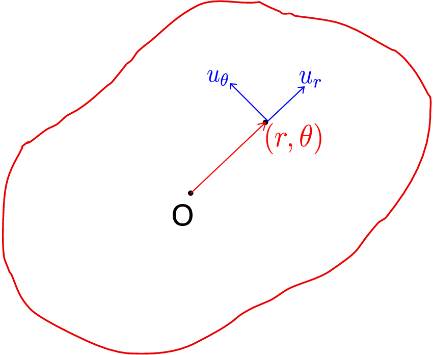
A point with coordinates (\(r,\theta \)) is also shown. After deformation of the body, displacement of this point in radial direction is \(u_r\), displacement in \(\theta \)-direction is \(u_\theta \) and displacement in \(z\)-direction (coming out of the plane) is \(u_z\). Now, we can plug in the displacement vector given in equation \eqref{7_u_cylindrical} in the gradient definition \eqref{7_gradient_cylindrical} to obtain the following:
For \({\partial }/{\partial r}\) and \({\partial }/{\partial z}\) terms here, the basis vectors act as a constant as they change only with \(\theta \). The derivatives of basis vectors with respect to \(\theta \) were derived earlier which when substituted in the above equation yields
We have gotten two extra terms here due to change in basis vectors. Let us use the above expression to obtain the displacement gradient matrix in cylindrical coordinate system. As the coefficient of the basis tensor \(\underline {e}_i\otimes \underline {e}_j\) goes into \(i^{th}\) row and \(j^{th}\) column, we obtain \begin {equation*} \hspace {40mm}r\hspace {18mm}\theta \hspace {15mm}z\hspace {1cm} \end {equation*} \begin {equation} \begin {bmatrix} \underline {\nabla }\,\underline {u} \end {bmatrix}_{(r,\theta ,z)}=~~ \begin {matrix} \, r\\\\\\ $\theta $\\\\\\ z \end {matrix}~~~ \begin {bmatrix} \dfrac {\partial u_r}{\partial r} & \dfrac {1}{r}\bigg (\dfrac {\partial u_r}{\partial \theta }-u_\theta \bigg ) & \dfrac {\partial u_r}{\partial z}\\\\ \dfrac {\partial u_\theta }{\partial r} & \dfrac {1}{r}\bigg (\dfrac {\partial u_\theta }{\partial \theta }+u_r\bigg ) & \dfrac {\partial u_\theta }{\partial z}\\\\ \dfrac {\partial u_z}{\partial r} & \dfrac {1}{r}\dfrac {\partial u_z}{\partial \theta } & \dfrac {\partial u_z}{\partial z} \end {bmatrix}. \end {equation}
Now, we can use equation \eqref{7_strain_displacement} to obtain strain matrix which is the symmetric part of displacement gradient matrix derived above. It turns out to be \begin {equation} \label {strain_cycs} \begin {bmatrix} \underline {\underline {\epsilon }} \end {bmatrix}_{(r,\theta ,z)}= \begin {bmatrix} \dfrac {\partial u_r}{\partial r} & \dfrac {1}{2}\Bigg [\dfrac {1}{r}\bigg (\dfrac {\partial u_r}{\partial \theta }-u_\theta \bigg )+\dfrac {\partial u_\theta }{\partial r}\Bigg ] & \dfrac {1}{2}\bigg (\dfrac {\partial u_r}{\partial z}+\dfrac {\partial u_z}{\partial r}\bigg )\\\\ \dfrac {1}{2}\Bigg [\dfrac {1}{r}\bigg (\dfrac {\partial u_r}{\partial \theta }-u_\theta \bigg )+\dfrac {\partial u_\theta }{\partial r}\Bigg ] & \dfrac {1}{r}\bigg (\dfrac {\partial u_\theta }{\partial \theta }+u_r\bigg ) & \dfrac {1}{2}\bigg (\dfrac {\partial u_\theta }{\partial z}+\dfrac {1}{r}\dfrac {\partial u_z}{\partial \theta }\bigg )\\\\ \dfrac {1}{2}\bigg (\dfrac {\partial u_r}{\partial z}+\dfrac {\partial u_z}{\partial r}\bigg ) & \dfrac {1}{2}\bigg (\dfrac {\partial u_\theta }{\partial z}+\dfrac {1}{r}\dfrac {\partial u_z}{\partial \theta }\bigg ) & \dfrac {\partial u_z}{\partial z} \end {bmatrix}. \end {equation}
The formulas of strain components (\(\epsilon _{rr},\epsilon _{zz},\epsilon _{rz},\epsilon _{\theta z}\)) are quite intuitive while the remaining strain components have unusual terms. The quantity \(\epsilon _{rz}\) gives us half of shear strain between line elements along \(\underline {e}_r\) and \(\underline {e}_z\), \(\epsilon _{\theta z}\) gives us half of shear strain between line elements along \(\underline {e}_\theta \) and \(\underline {e}_z\) and \(\epsilon _{zz}\) gives us longitudinal strain of a line element directed along \(\underline {e}_z\). Let us now develop a physical understanding of other strain components.
\begin {equation} \epsilon _{rr}=\Big (\underline {\underline {\epsilon }}\,\underline {e}_r\Big )\cdot \underline {e}_r=\frac {\partial u_r}{\partial r}. \end {equation} This is called radial longitudinal strain or simply radial strain. To visualize this, we can think of a typical cross-section of a hollow cylinder as shown in Figure 7.7.
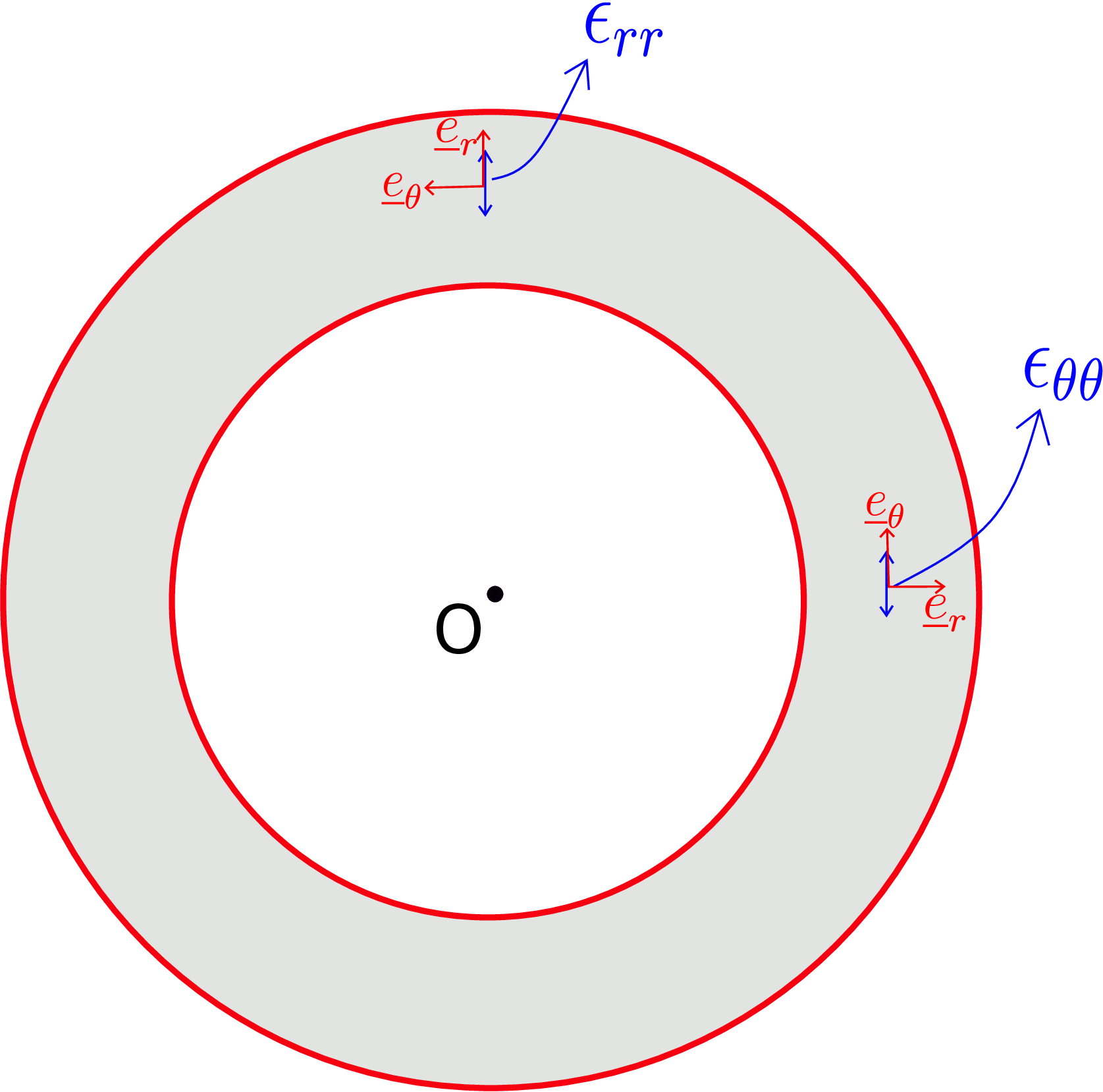
The elongation of a radial line element generates \(\epsilon _{rr}\) as shown.
\begin {equation} \label {7_epsilon_theta_theta} \epsilon _{\theta \theta }=\Big (\underline {\underline {\epsilon }}\,\underline {e}_\theta \Big )\cdot \underline {e}_\theta =\frac {1}{r}\bigg (\frac {\partial u_\theta }{\partial \theta }+u_r\bigg ). \end {equation} This strain is also called hoop strain or circumferential strain. This is the elongation of a line element directed along \(\theta \)-direction (circumferential line element) as shown in Figure 7.7. The circumferential strain has two contributions. The partial derivative term is intuitive because longitudinal strain along a direction is understood as the derivative of displacement in that direction with respect to distance in the same direction. The other term \(\dfrac {u_r}{r}\) is the unusual term which we now try to understand physically. Think of a displacement which has only radial component, i.e.,
For such a displacement, if we find \(\epsilon _{\theta \theta }\) using equation \eqref{7_epsilon_theta_theta}, we will get \begin {equation} \epsilon _{\theta \theta }=\frac {u_r}{r}\neq 0. \end {equation} Figure 7.8 again shows a typical cross section of a hollow cylinder. For the displacement given in \eqref{7_Hoop_example}, all points in the cross-section simply displace radially.
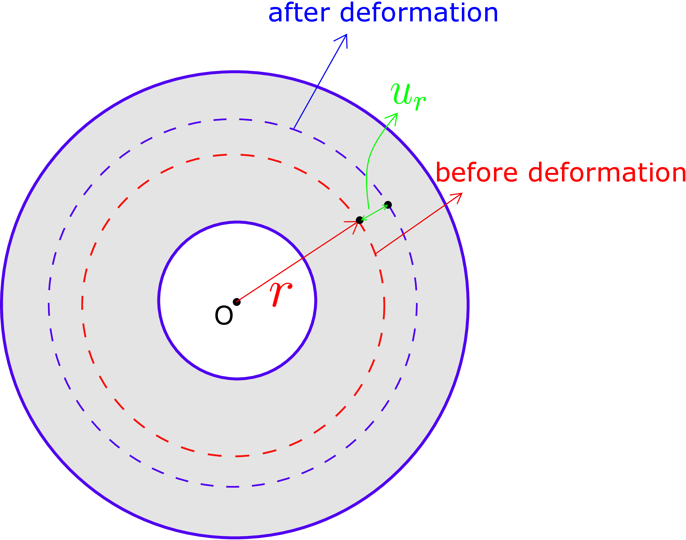
We have also drawn a circumferential line both before and after deformation. All points on this line initially at radial coordinate \(r\) displace to radial coordinate \(r+u_r\). We can notice that the length of the original circumferential line (shown in red) has increased generating longitudinal strain in it, i.e.,
which by definition is \(\epsilon _{\theta \theta }\). This specific case shows that despite \(u_\theta \) being zero, the extra term in \(\epsilon _{\theta \theta }\) generates non-zero hoop strain.
We can see from the strain matrix that we have an extra term in \(\epsilon _{r\theta }\) also, i.e., \begin {equation} \gamma _{r\theta }=2\epsilon _{r\theta }=2\Big (\underline {\underline {\epsilon }}\,\underline {e}_r\Big )\cdot \underline {e}_\theta =\dfrac {1}{r}\bigg (\dfrac {\partial u_r}{\partial \theta }-u_\theta \bigg )+\dfrac {\partial u_\theta }{\partial r}. \end {equation} This denotes the change in angle between two initially perpendicular line elements directed along \(\underline {e}_r\) and \(\underline {e}_\theta \).
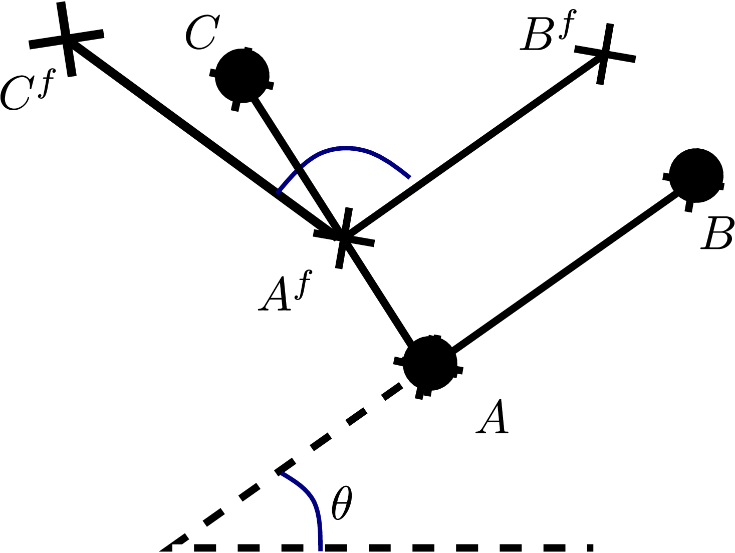
Let us try to figure out the origin of unusual term in \(\gamma _{r\theta }\). Think of a simple displacement such that \(u_r = u_z = 0\) but \(u_{\theta }\) is a non-zero constant, i.e., \(\underline {u} = u_{\theta }~\underline e_{\theta }(\theta )\). Notice that although the coefficient \(u_{\theta }\) is assumed constant but \(\underline {u}\) is not because \(\underline e_{\theta }\) changes with \(\theta \). At an arbitrary point \((r,\theta ,z)\), we consider two line elements directed along \(\underline {e}_r\) and \(\underline {e}_\theta \) respectively (see Figure 7.9): \(\overrightarrow {AB}\) is the radial line element, \(\overrightarrow {AC}\) is the circumferential line element and the three points there have the following position vectors: \begin {equation} \overrightarrow {A} = r~\underline e_{r}(\theta ),\quad \overrightarrow {B} = (r + \Delta r)~\underline e_{r}(\theta ),\quad \overrightarrow {C} = r~\underline e_{r}(\theta + \Delta \theta ). \end {equation} Keep in mind that the two line elements are infinitesimally small in length - they are just shown as being of finite length for clarity. After displacement, the three points move to (also see Figure 7.9) \begin {equation} \overrightarrow {A}^f = r\underline e_{r}(\theta ) + u_{\theta }\underline e_{\theta }(\theta ),\quad \overrightarrow {B}^f = (r + \Delta r)\underline e_{r}(\theta ) + u_{\theta }\underline e_{\theta }(\theta ),\quad \overrightarrow {C}^f = r\underline e_{r}(\theta + \Delta \theta ) + u_{\theta }\underline e_{\theta }(\theta + \Delta \theta ). \end {equation} Accordingly, \begin {align} \overrightarrow {AB}^f &= \overrightarrow {B}^f - \overrightarrow {A}^f = \Delta r\underline e_{r}(\theta ) = \overrightarrow {AB},\nonumber \\ \overrightarrow {AC}^f &= \overrightarrow {C}^f - \overrightarrow {A}^f = r\underline e_{r}(\theta + \Delta \theta ) + u_{\theta }\underline e_{\theta }(\theta + \Delta \theta ) - r\underline e_{r}(\theta ) + u_{\theta }\underline e_{\theta }(\theta )\nonumber \\ &= r\frac {\partial \underline e_{r}}{\partial \theta }\Delta \theta + u_{\theta }\frac {\partial \underline e_{\theta }}{\partial \theta }\Delta \theta + h.o.t.\approx r\Delta \theta ~\underline e_{\theta } - u_{\theta }\Delta \theta ~\underline e_{r}. \end {align}
Notice that the radial line element has not changed its orientation but the circumferential line element has. Thus, the final angle between the two line elements is \begin {align} & \cos {\theta }^f = \frac {\overrightarrow {AB}^f\cdot \overrightarrow {AC}^f}{||\overrightarrow {AB}^f||\;||\overrightarrow {AC}^f||} = \frac {\Delta r \underline e_{r}\cdot (r\Delta \theta ~\underline e_{\theta } - u_{\theta }\Delta \theta ~\underline e_{r})}{\Delta r~r\Delta \theta \sqrt {1+\frac {u_{\theta }^2}{r^2}}} \approx -\frac {u_{\theta }}{r}\nonumber \\ &\Rightarrow \sin {(90-\theta ^f)} = -\frac {u_{\theta }}{r}\quad \text {or shear strain} = -\frac {u_{\theta }}{r}. \end {align}
Basically, the unusual term arises because \(u_{\theta }\) is in different direction for different points!
Once we have stress and strain matrices in cylindrical coordinate system, let us relate them for an isotropic material. We know how to relate stress and strain in Cartesian coordinate system. We also know that for an isotropic material, the material properties are independent of direction. Thus, the relationship between stress and strain components must also be independent of the coordinate system. This means that we could choose any set of three perpendicular directions and resolve our stress and strain tensors in those directions but the mathematical form of their relationship would remain unchanged. For example: \begin {equation} \epsilon _{11}=\frac {1}{E}(\sigma _{11}-\nu (\sigma _{22}+\sigma _{33}))\Rightarrow \epsilon _{rr}=\frac {1}{E}(\sigma _{rr}-\nu (\sigma _{\theta \theta }+\sigma _{zz})). \end {equation} We can obtain all other relations in a similar way leading to
Having obtained stress and strain components and their relation in cylindrical coordinate system, we will learn next how using them leads to simplified form of equations when studying axisymmetric deformation of cylindrical bodies. Such problems could also be solved in Cartesian coordinate system but the equations would not simplify then.
We will now study three special cases of deformation, i.e., extension, torsion and inflation which generate axisymmetric deformation in cylinders. If we apply axial force to a cylinder by applying normal traction on its two end cross-sections as shown in Figure 7.10, the cylinder gets stretched.
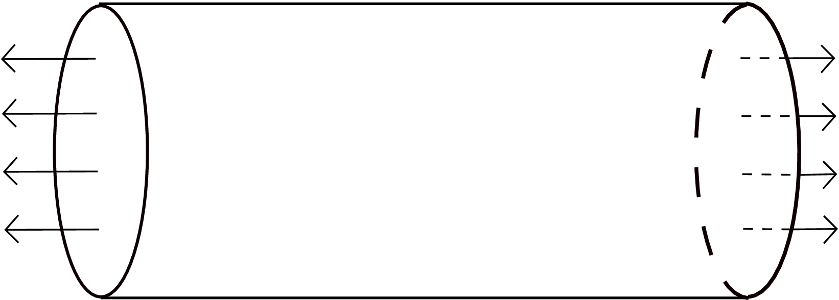
Such deformations are called extension. On the other hand, if we hold the two ends of a cylinder and rotate them in opposite directions as shown in Figure 7.11, different cross-sections of the cylinder rotate by different angle.
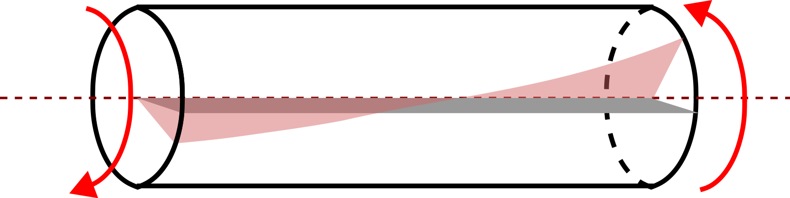
Such a deformation is called twisting or torsion of a cylinder. Finally, if we pressurize a hollow cylinder from within its inner cavity as shown in Figure 7.12, the inner and outer radii of the cylinder change. It has application in modeling of pressure vessels.
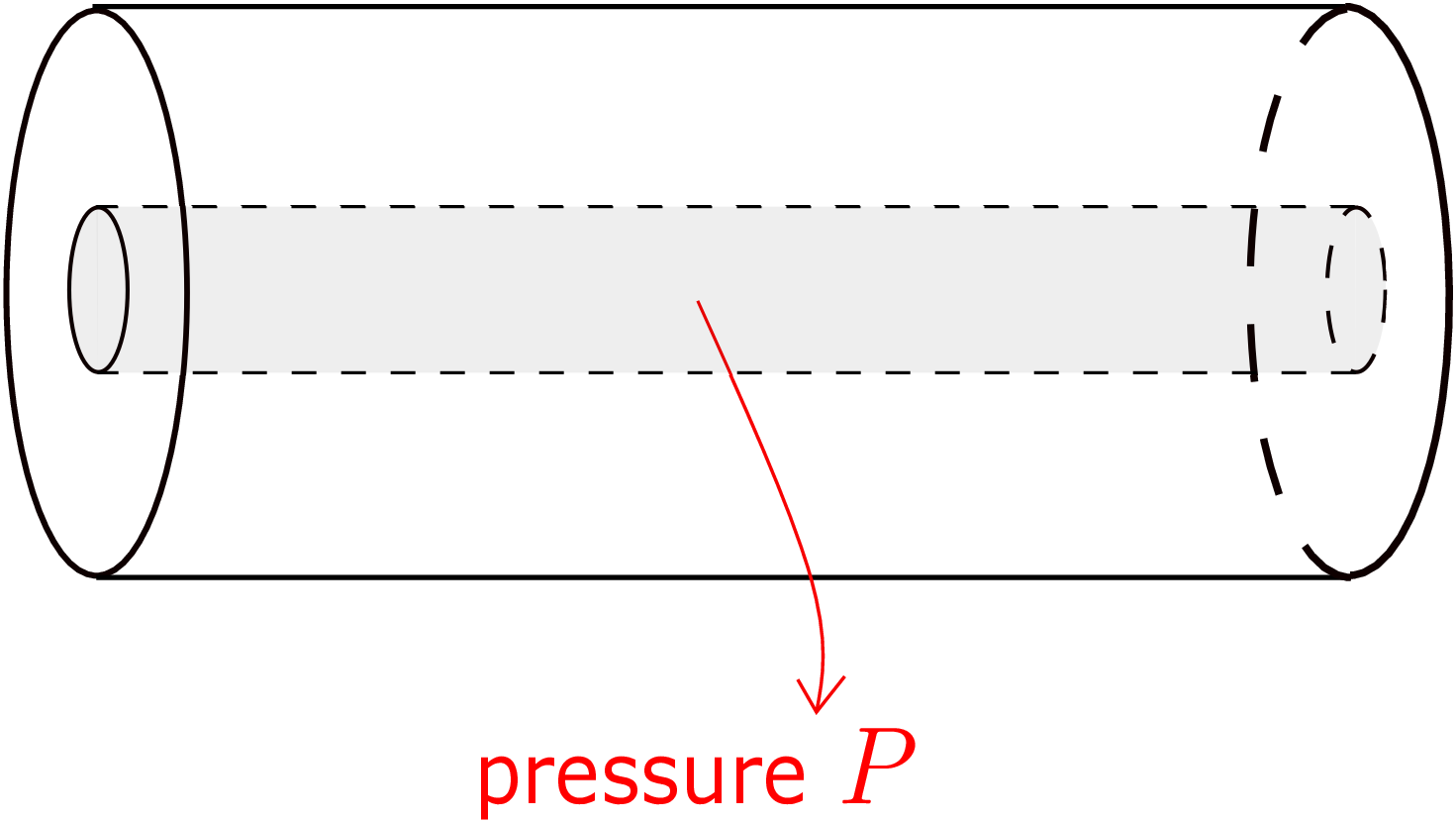
Such deformations are called inflation. Let us develop a mathematical formulation for the deformation of a cylinder when it is subjected to combined axial load, torque and internal pressure. Note that the stress components are proportional to strain components and strain components are proportional to displacement components. This implies that the governing equations being linear in stress components, also become linear in unknown displacement components. Likewise, the boundary conditions also become linear in the unknowns. As a whole, we therefore call it linear elasticity. This linearity allows us to use the principle of superposition, i.e., we can obtain solution to extension, torsion and inflation problems individually and finally combine the individual solutions to obtain solution to the combined loading problem.¶ Nevertheless, we will investigate this problem in a combined manner here for the sake of the brevity of presentation.
Let us consider a hollow cylinder subjected to an axial force F, torque T and internal pressure P as shown in Figure 7.13.ʺ
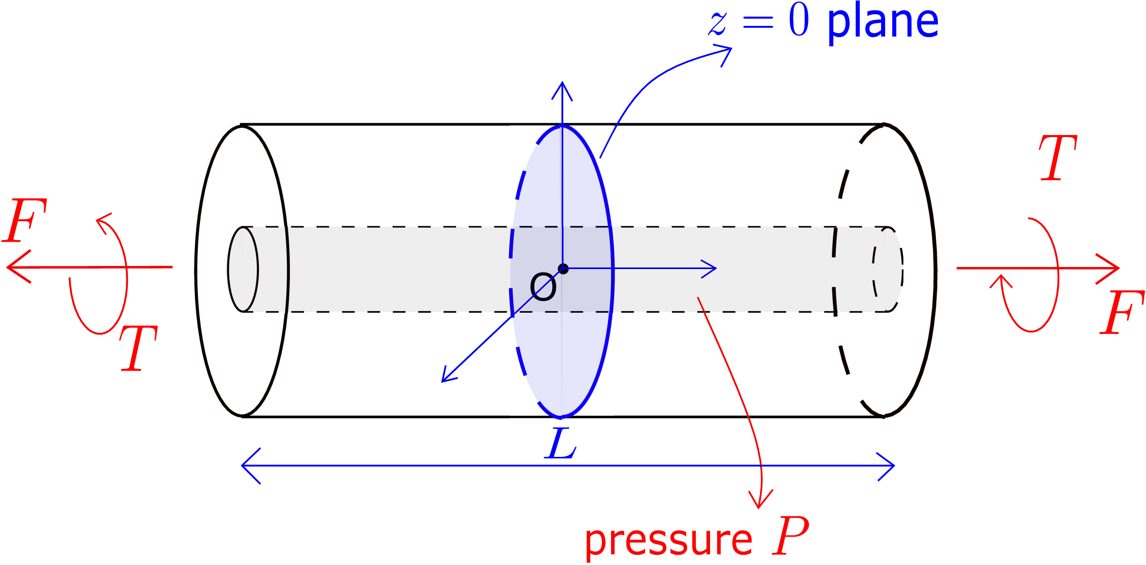
Our goal is to find all the displacement and stress components that generate in the cylinder.
Before we start solving the problem mathematically, let us simplify it using physical considerations. The displacement \(\underline {u}\) is given by \begin {equation} \underline {u}=u_r\underline {e}_r+u_\theta \underline {e}_\theta +u_z\underline {e}_z \end {equation} where each of the displacement components is a function of \(r\), \(\theta \) and \(z\), i.e.,
However, as we are analyzing a special deformation here, some of the dependencies on \(r\), \(\theta \) and \(z\) won’t be there as we show now.
We can imagine that upon applying axial force, torque and pressure to an axisymmetric cylinder, the deformation induced would also be axisymmetric. This automatically implies that none of the displacement components depend on \(\theta \), i.e., if we consider any two points in the cylinder with the same \(r\) and \(z\) coordinates but different \(\theta \) coordinate, the displacement components at the two points must be the same. If \(u_r\) depends on \(\theta \), a circular cross-section will not remain circular after deformation voilating axisymmetry (see Figure 7.14).
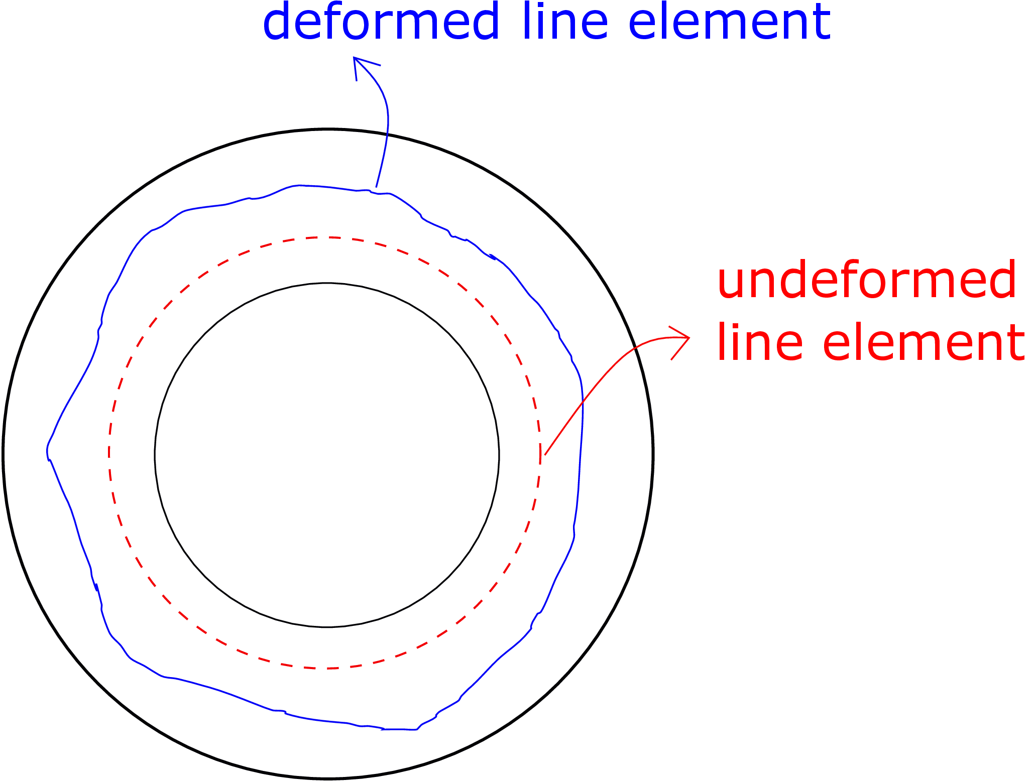
Similarly, if \(u_\theta \) or \(u_z\) changes with \(\theta \), axisymmetry will be lost. Thus, using axisymmetry, we can write
If \(u_r\) is a function of \(z\), homogeneity along the axis will be lost.
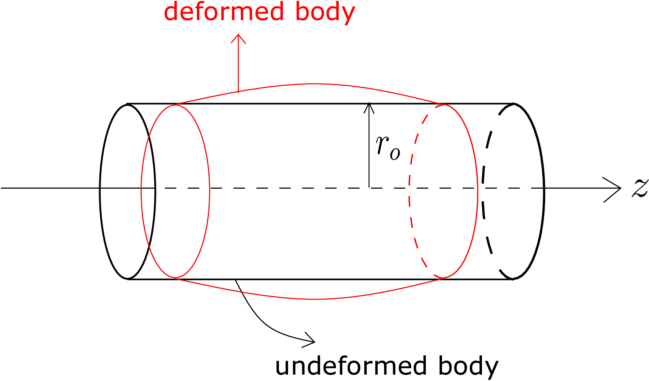
Figure 7.15 displays such a case where a simple cylinder (constant radius along the axis) with outer radius \(r_o\) is shown in black. If \(u_r\) changes with \(z\), the final radius of the cylinder at different locations along the axis will be different and the deformed configuration (shown in red) will no more be a simple cylinder. This is usually the case when we compress a cylinder while holding the end cross-sections tightly: the two end cross-section radii do not change but the radius of the cross-sections between the two ends increase due to Poisson’s effect. The analysis of such a deformation is more difficult. We will instead consider a a simpler case where we allow the end cross-sections to also relax. In such a case, all the cross-sections of the cylinder will undergo the same change in radius giving us an axially homogeneous deformed configuration. Thus, \(u_r\) would be independent of \(z\), i.e, \begin {equation} u_r(r,z)\xRightarrow {\text {axial homogeneity}} u_r(r). \end {equation}
Let us think of the cylinder again and consider its planar cross-section. All the points in the cross-section have the same \(z\) coordinate. The displacement component \(u_z\) displaces these points in the axial direction. If \(u_z\) changes with \(r\), two points on a typical cross-section (having different radial coordinate) would displace in the axial direction by different amounts. This will make the deformed cross section non-planar which is also called warping. We assume no such warping occurs. So, \(u_z\) must be independent of \(r\), i.e., \begin {equation} u_z(r,z)\xRightarrow {\text {no warping}} u_z(z) \end {equation}
We also have some restriction on \(u_\theta \) which we explain now. The extension of a cylinder generates both axial and radial (due to Poisson’s effect) components of displacement but no \(u_{\theta }\) for isotropic tubes. Similarly, by applying internal pressure, we can generate radial and axial displacements (due to Poisson’s effect) but no \(u_\theta \) again for isotropic cylinders. An application of torque, on the other hand, causes a typical cross-section to rotate which only generates \(u_\theta \) for isotropic tubes.∗∗ To quantify this displacement, let us consider a cross-section of the cylinder which rotates by an angle \(\alpha \) (see Figure 7.16).
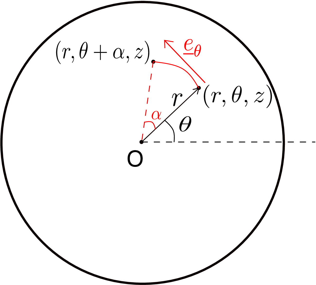
An arbitrary point on the cross section having initial coordinate (\(r,\theta ,z\)) displaces to (\(r,\theta +\alpha ,z\)). The arc of rotation of the point under consideration is shown as a solid red curve whose length equals \(r\alpha \). This arc would become a straight line in \(\underline {e}_\theta \) direction when \(\alpha \) is very small. Thus, we get \begin {equation} \label {7_u_theta_alpha} u_\theta =\alpha (z)~ r\text { (if $\alpha $ is very small)}. \end {equation} We can observe that \(u_\theta \) is independent of \(\theta \) as required due to axisymmetry. We have finally simplified our displacement functions to
Let us now obtain the strain matrix. Upon substituting the simplified displacement components \eqref{7_simplified_u} in \eqref{strain_cycs}, we get \begin {equation} \label {7_simplified_strain} \begin {bmatrix} \underline {\underline {\epsilon }} \end {bmatrix}_{(r,\theta ,z)}= \begin {bmatrix} u'_r & \, & 0 & \, & 0\\\\ 0 & \, & \dfrac {u_r}{r} & \, & \dfrac {\alpha ' r}{2}\\\\ 0 & \, & \dfrac {\alpha ' r}{2} & \, & u'_z \end {bmatrix}. \end {equation} Note that the only shear strain that is non-zero is \(\gamma _{\theta z}\) - it arises due to torsion.
Substituting strain components from \eqref{7_simplified_strain} in isotropic stress-strain relation, we get
Let us now substitute the above stress components in the below equations of equilibrium:
Most of the terms in the above equations become zero which simplifies the equations to††
If we had used Cartesian coordinate system, this simplification would not have been possible. Let us now consider some simple axisymmetric deformation examples and find out the corresponding body force components and acceleration components.
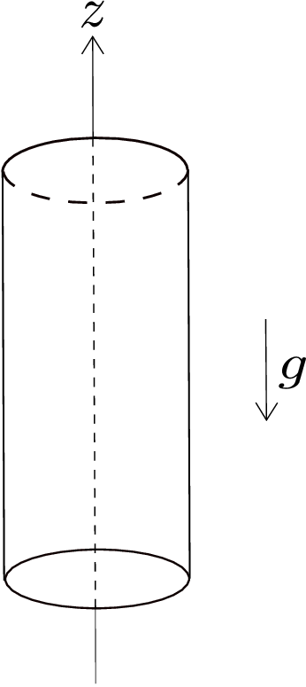
When the cylinder is vertical and \(g\) acts along the axis of the cylinder as shown in Figure 7.17, the body force components would be
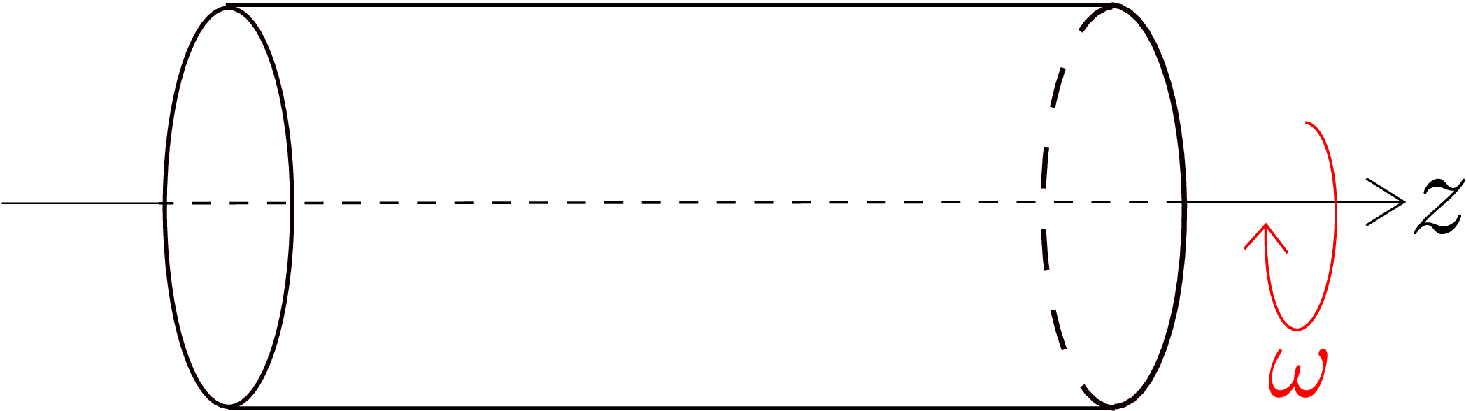
If the cylinder rotates about its axis with a constant angular speed \(\omega \) as shown in Figure 7.18, it will have centripetal acceleration of magnitude \(\rho \omega ^2r\) acting in the radially inward direction, i.e.,‡‡
There is no body force in this case if we neglect gravity. If we sit on the rotating shaft itself and analyze its deformation, we need to apply pseudo force, i.e., centrifugal force to use Newton’s second law. Thus, a body force in the radially outward direction replaces the radial acceleration component, i.e,
In both the view points, the radial equation of equilibrium becomes \begin {equation} \frac {\partial \sigma _{rr}}{\partial r}+\frac {\sigma _{rr}-\sigma _{\theta \theta }}{r}+\rho \omega ^2 r=0. \end {equation}
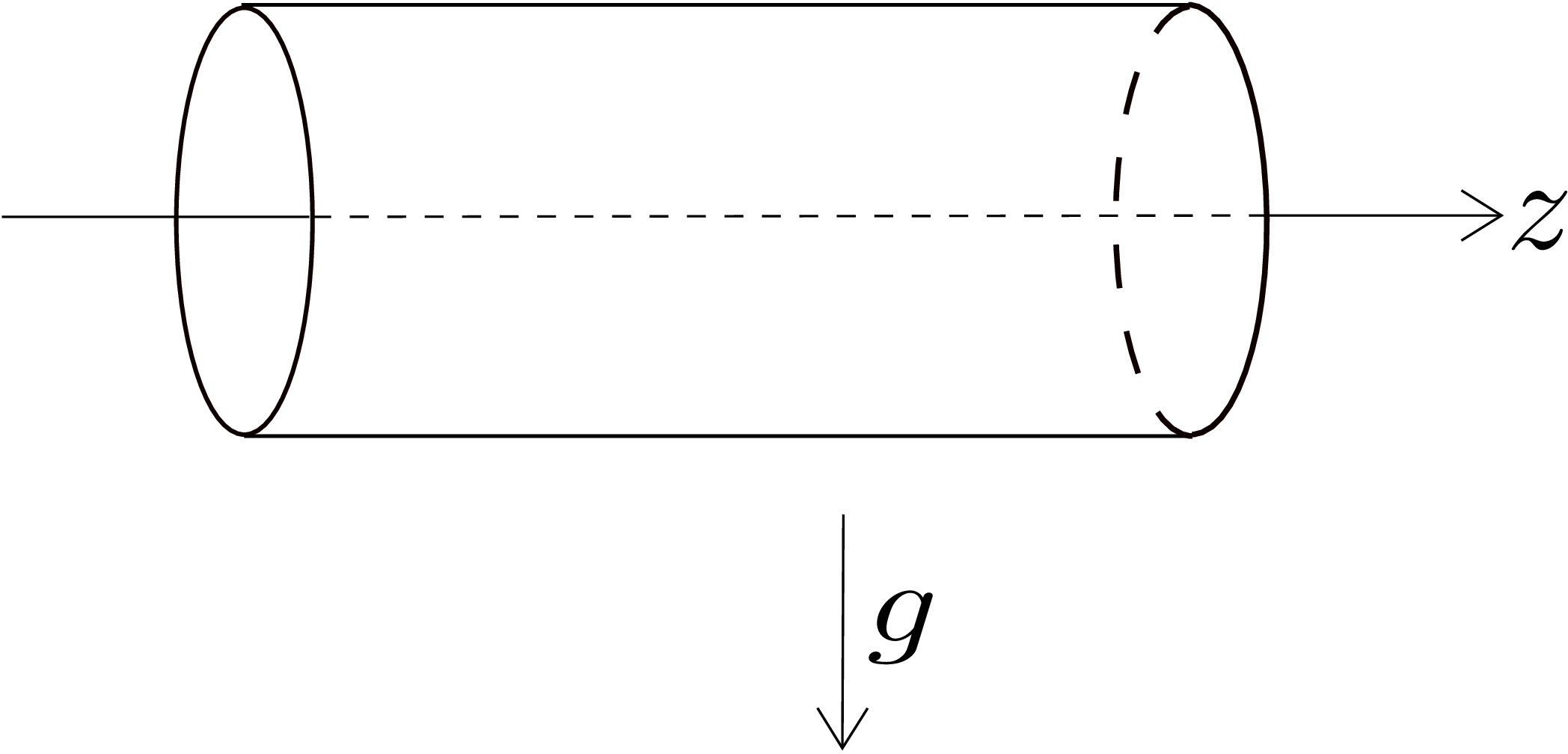
If the axis of the cylinder is horizontal and gravity acts vertically downwards as shown in Figure 7.19, the body force components (\(b_r\) and \( b_\theta \)) will become function of \(\theta \) as shown below:
This breaks our axisymmetric assumption.
For the original problem where only axial force \(F\), torque \(T\) and internal pressure \(P\) are applied, all body force components will be zero.§§ If it is also a statics problem, all the acceleration components will be zero too. Setting all body force and acceleration components to zero in \eqref{7_equilibium_before_final}, the final simplified set of equations for extension-torsion-inflation problem would be
We can solve these to obtain the unknown displacement components (\(u_r,u_z\)) and also the variable \(\alpha \). Concerning \(\alpha \), the second equation above implies \(\alpha '\) is a constant or the angle \(\alpha \) by which every cross-section rotates varies linearly in \(z\). Let us now write \(\alpha \) in terms of end-to-end rotation \(\Omega \). If the right most cross-section rotates by \(\dfrac {\Omega }{2}\) in one direction while the leftmost cross-section rotates by \(\dfrac {\Omega }{2}\) in the other direction (see Figure 7.11), then
Here we have assumed that z=0 lies at the mid-section of the cylinder where the cross-section does not rotate. The quantity \(\alpha '\) is also called twist. Plugging the above form for \(\alpha \) into equation \eqref{7_u_theta_alpha}, we get \begin {equation} \label {7_u_theta} u_\theta =\frac {\Omega }{L}rz. \end {equation} Thus, the mathematical form of \(u_{\theta }\) gets fully determined.
As \(u_z\) and \(u_r\) are functions of \(z\) and \(r\) respectively, we can rewrite equation \eqref{7_constitutive_sigma_zz} as \begin {equation} \sigma _{zz}=\underbrace {(\lambda +2\mu )u'_z}_{\text {depends on $z$}}+\underbrace {\lambda \Big (u'_r+\frac {u_r}{r}\Big )}_{\text {depends on $r$}}. \end {equation} Notice that \(\sigma _{zz}\) does not have any dependence on \(\theta \). Also from the third equation in \eqref{7_simplified_eq_axisym}, we can infer that \(\sigma _{zz}\) does not depend on \(z\). Thus, it is a function of \(r\) only, i.e., \begin {equation} \underbrace {(\lambda +2\mu )u'_z}_{\text {depends on $z$}}+\underbrace {\lambda \Big (u'_r+\frac {u_r}{r}\Big )}_{\text {depends on $r$}}=f(r). \end {equation} Accordingly, the term dependent on \(z\) in the LHS must be a constant or \(u'_z\) is a constant. As \(u'_z\) denotes the longitudinal strain in axial direction, we will denote it by \(\epsilon \): an unknown parameter. Upon integrating \(u_z'=\epsilon \), we finally get \begin {equation} u_z=\epsilon z. \end {equation} Here we have assumed that \(u_z\) vanishes when \(z=0\) where the cylinder’s mid-section lies. In order to obtain an expression for \(u_r\), we look at the radial component of equilibrium equation. The expressions of \(\sigma _{rr}\) and \(\sigma _{\theta \theta }\) given in \eqref{7_constitutive_sigma_rr} and \eqref{7_constitutive_sigma_theta theta} now become
Subtracting them, we get \begin {equation} \label {7_sigma_rr_minus_sigma_theta_theta} \sigma _{rr}-\sigma _{\theta \theta }=2\mu \Big (u'_r-\frac {u_r}{r}\Big ). \end {equation} Likewise, taking the partial derivative of equation \eqref{7_constitutive_sigma_rr2} with respect to \(r\), we get \begin {equation} \label {7_del_sigma_rr_by_r} \frac {\partial \sigma _{rr}}{\partial r}=\lambda \Big (u'_r+\frac {u_r}{r}\Big )'+2\mu u''_r. \end {equation} Now, we can plug equations \eqref{7_sigma_rr_minus_sigma_theta_theta} and \eqref{7_del_sigma_rr_by_r} into the first equation in \eqref{7_simplified_eq_axisym} to get
We can infer from this that \(\Big (u'_r+\dfrac {u_r}{r}\Big )\) is also a constant, say \(C\). Further, from the definition of strain components, we know that \(\epsilon _{rr}=u'_r\) and \(\epsilon _{\theta \theta }=\dfrac {u_r}{r}\). Thus, we get \begin {equation} \label {7_sum_eps_rr_eps_theta_theta} \boxed {u'_r+\dfrac {u_r}{r}=\epsilon _{rr}+\epsilon _{\theta \theta }=C} \end {equation} Integrating \eqref{7_before_complete_derivative} twice, we finally get
where \(C\) and \(D\) are the unknown integrating constants. These constants can be obtained by applying the boundary condition at inner and outer radii of the cylinder.
Let us add equations \eqref{7_constitutive_sigma_rr2} and \eqref{7_constitutive_sigma_theta_theta2}:
Thus, the sum of radial and hoop stresses turns out to be a constant through the thickness of the tube although they vary individually. Let us now solve the radial equilibrium equation in \eqref{7_simplified_eq_axisym} directly in terms of stress components as follows:
Notice that the partial derivative above has become total derivative since we now know that \(\sigma _{rr}\) is just a function of \(r\). Continuing further, we get
Here \(A\) and \(B\) are the unknown integrating constants. Let us now use boundary condition to obtain these constants.
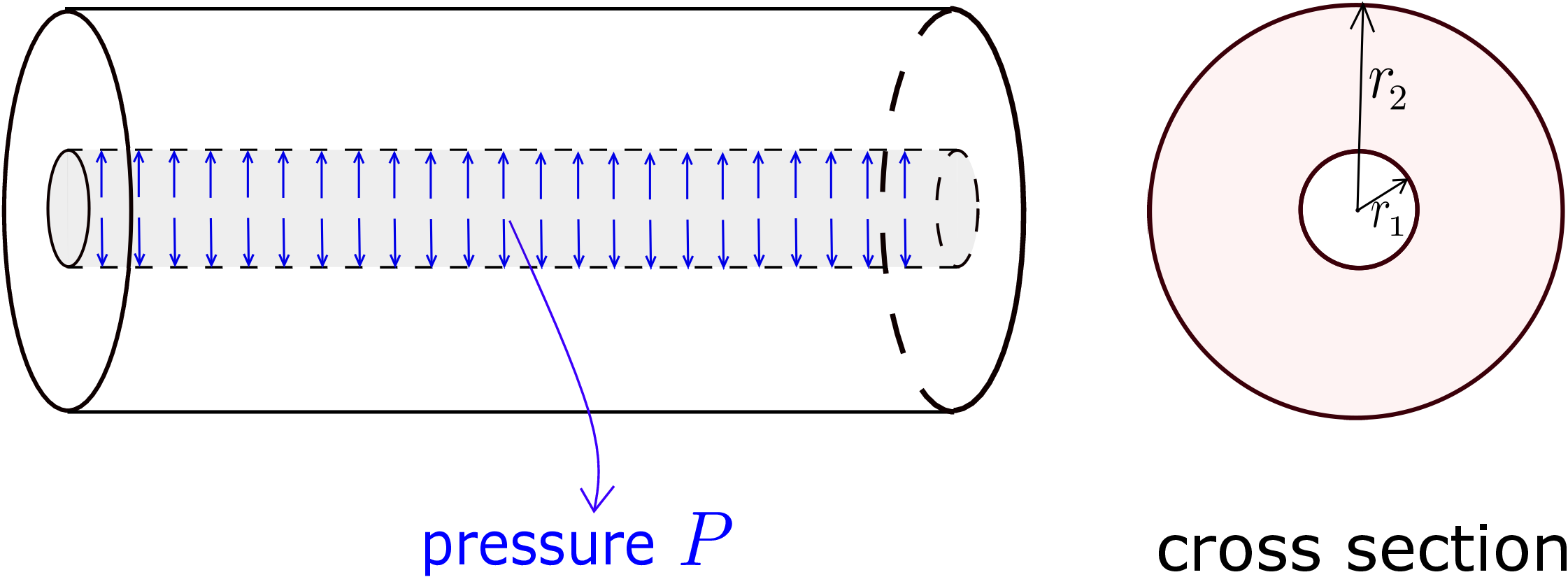
Figure 7.20 shows a cylinder subjected to some internal pressure on its inner surface and zero traction on its outer surface. The outward surface normal of the inner curved surface (at \(r=r_1\)) points in \(-r\) direction, i.e., \begin {equation} \begin {bmatrix} \underline {n} \end {bmatrix}_{(r,\theta ,z)}= \begin {bmatrix} -1\\0\\0 \end {bmatrix} \end {equation} while the pressure traction there acts in \(+r\) direction, i.e., \begin {equation} \begin {bmatrix} \underline {t}^{\text {ext}} \end {bmatrix}_{(r,\theta ,z)}= \begin {bmatrix} P\\0\\0 \end {bmatrix}. \end {equation} Upon writing the boundary condition \(\underline {\underline {\sigma }}~\underline {n}=\underline {t}^{\text {ext}}\) at the inner surface in cylindrical coordinate system, we get
Similar analysis for the outer surface where no external traction is present yields
We have thus obtained the following two boundary conditions to obtain the unknown integrating constants in the expression of \(\sigma _{rr}\): \begin {equation} \label {bc_sigmarr} \sigma _{rr}(r_1)=-P,\quad \sigma _{rr}(r_2)=0. \end {equation} Upon plugging them in equation \eqref{7_sigma_rr_before_constants}, we get the following set of equations:
solving which we get
For a positive internal pressure \(P\), we always have \(A>0\) and \(B<0\). Using \eqref{7_sigma_rr_before_constants}, we can now plot the variation in both \(\sigma _{rr}\) and \(\sigma _{\theta \theta }\) through the tube’s thickness as shown in Figure 7.21.
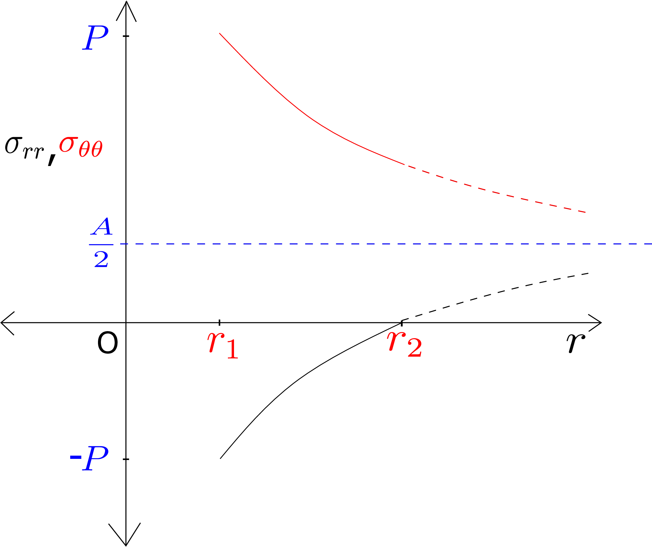
The red curve shows the variation of \(\sigma _{\theta \theta }\) while the black curve shows the variation of \(\sigma _{rr}\). As \(r\to \infty \), both \(\sigma _{rr}\) and \(\sigma _{\theta \theta }\) approach \({A}/{2}\) (see the blue dashed line in Figure 7.21) which is a positive number.¶¶ Furthermore, as the sum of \(\sigma _{rr}\) and \(\sigma _{\theta \theta }\) is \(A\), the curve for \(\sigma _{\theta \theta }\) is the mirror image of \(\sigma _{rr}\) about the blue dashed line. Lastly, \(\sigma _{rr}\) and \(\sigma _{\theta \theta }\) depend only on pressure \(P\) and radial coordinate as can be seen from equations \eqref{7_AB} and \eqref{7_sigma_rr_before_constants}. If there is no internal pressure, \(\sigma _{rr}\) and \(\sigma _{\theta \theta }\) will simply vanish even if axial force and twisting moment are present. This happens because the cross section is free to relax during extension and torsion of a circular cylinder.∗∗∗
To obtain the constants \((C,D)\) in expression \eqref{7_u_r_constants}, let us rewrite equation \eqref{7_constitutive_sigma_rr2} after substituting equation \eqref{7_u_r_constants} in it:
Comparing this with equation \eqref{7_sigma_rr_before_constants}, we get
Thus \(u_r\) finally becomes \begin {equation} \label {7_final_ur} \boxed {u_r=\Bigg (\frac {-\lambda }{2(\lambda +\mu )}\epsilon +\frac {P}{2(\lambda +\mu )}\,\frac {r_1^2}{r_2^2-r_1^2}\Bigg )r+\frac {P}{2\mu r}\frac {r_1^2 r_2^2}{r_2^2-r_1^2}.} \end {equation} In the special case when pressure is not acting, the above equation reduces to \begin {equation} u_r=\frac {-\lambda }{2(\lambda +\mu )}\epsilon r = -\nu \epsilon r \quad \left (\because \nu =\frac {\lambda }{2(\lambda +\mu )}\right ) \end {equation} and the radial longitudinal strain becomes \begin {equation} \epsilon _{rr}=u'_r=-\nu \epsilon . \end {equation} This is exactly what we would expect in the absence of pressure - radial displacement has arisen only due to Poisson’s effect. We need to finally obtain axial strain \(\epsilon \) and the end-to-end rotation \(\Omega \) in terms of prescribed external loads (axial force \(F\), Torque \(T\) and internal pressure \(P\)).
Typically, the ends of a cylinder are capped as in pressure vessels. In such a case, the end cap is pushed out by internal pressure \(P\) but pulled in by traction component \(\sigma _{zz}\). It is further pulled out by external load \(F\). Upon doing its force balance, we can then write
Upon further substituting \(C\) from \eqref{7_CD}, we finally obtain \begin {equation} F=\left [(\lambda +2\mu )-\frac {\lambda ^2}{\lambda +\mu }\right ]A \epsilon - \pi r^2_1 P \left (1-\frac {\lambda }{\lambda +\mu }\right ). \end {equation} Here \(A=\pi (r_2^2-r_1^2)\) is the cross-sectional area. Upon further noting that the Young’s modulus \(E=\frac {\mu (3\lambda +2\mu )}{\lambda +\mu }\) and the Poisson’s ratio \(\nu =\frac {\lambda }{2(\lambda +\mu )}\), the above expression simplifies to \begin {equation} F=EA \epsilon - \pi r^2_1 P \left (1-2\nu \right ). \end {equation} This expression relates axial strain \(\epsilon \) with the applied axial load and pressure.
A typical cross-section of a hollow cylinder is shown in Figure 7.22.
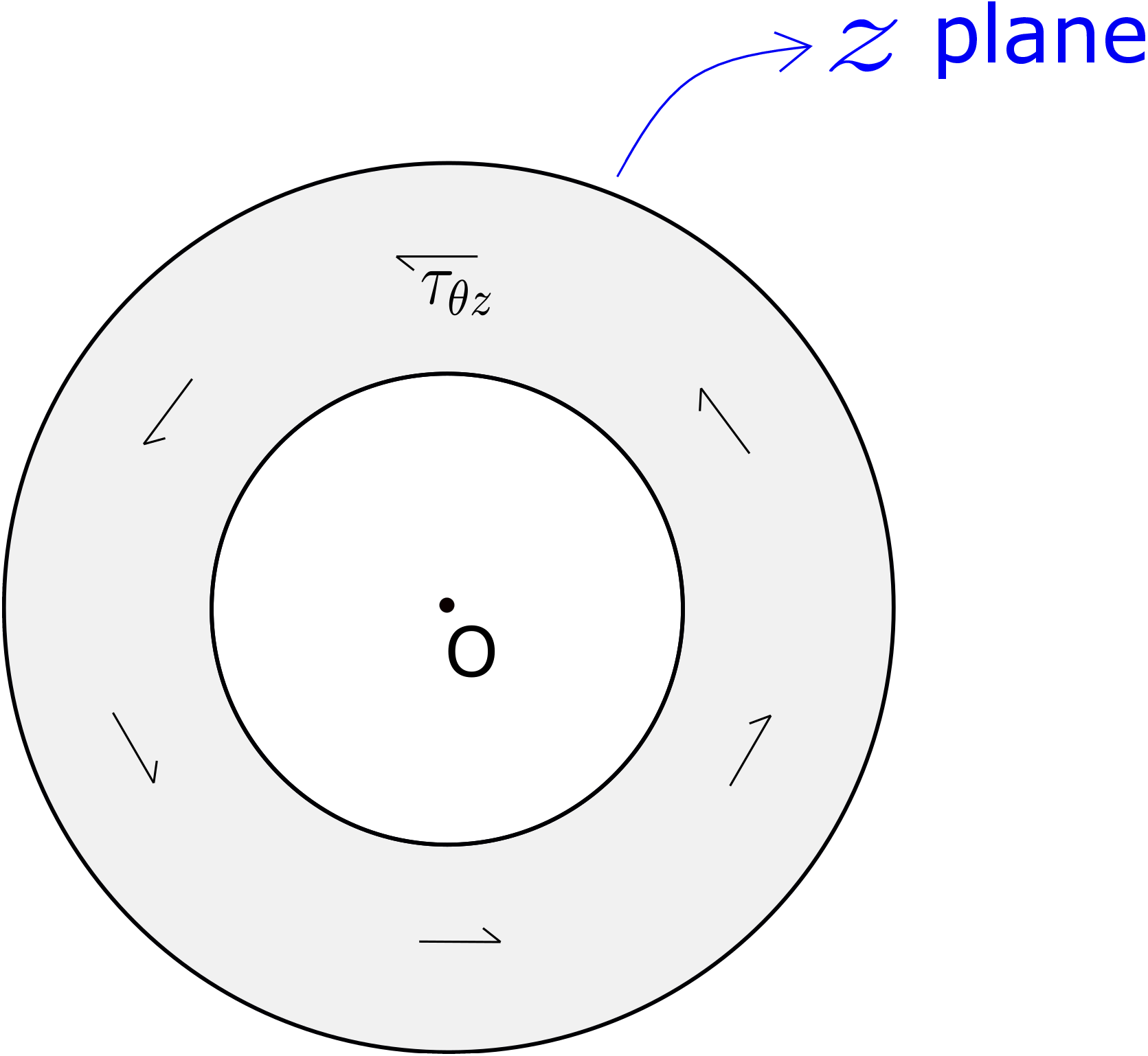
As the cross-section normal points along \(z\) direction, the stress components \(\sigma _{zz}\), \(\tau _{\theta z}\) and \(\tau _{rz}\) act on it. We had earlier found \(\tau _{rz}\) to be zero. Let \(\Omega _0\) denote the area of the cross section. The moment \(M\) about the cross-section’s centroid will be given by
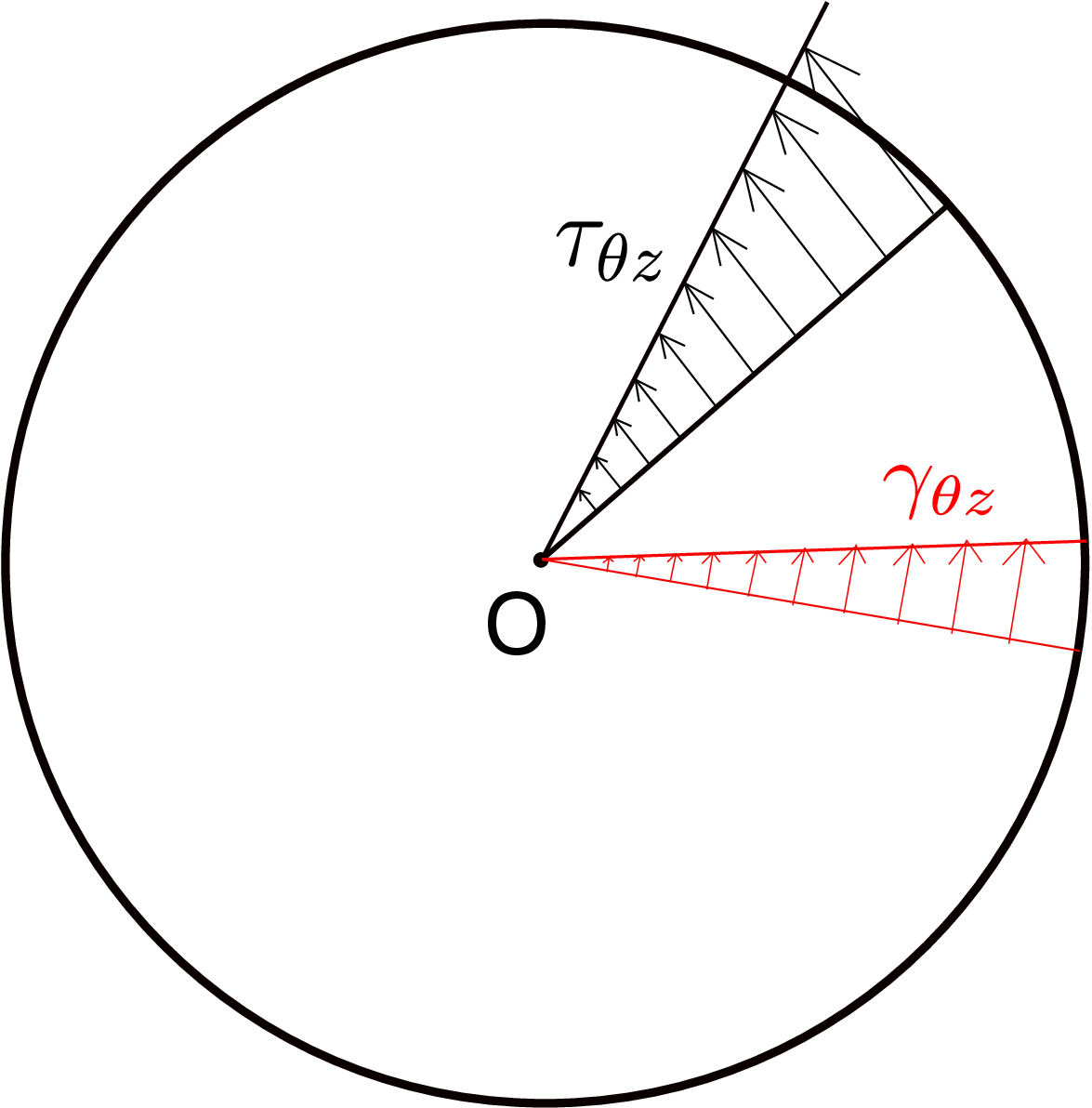
Before, we obtain torque from it, let us analyze graphically the variation in \(\tau _{\theta z}\) in the cross-section - we show later that this is responsible for generating torque. We know
This implies that both the quantities vary linearly with \(r\) (see Figure 7.23).
The torque \(T\) is simply the component of moment along the axis, i.e.,
The term \(\iint _{\Omega _0}r^2 dA\) is the polar moment of area (a geometric quantity) and is denoted by \(J\). Thus, we finally get \begin {equation} T=GJ\frac {\Omega }{L}~\text {or}~ \Omega =\frac {TL}{GJ}. \end {equation} We have finally derived the relationship between \(\Omega \) and \(T\) as well as the relationship between \(\epsilon \) and \(F\). The constant \(EA\) is called stretching stiffness while the constant GJ is called torsional stiffness. One can now write
We can also think of a composite cylinder made up of two different materials as shown in Figure 7.24a.
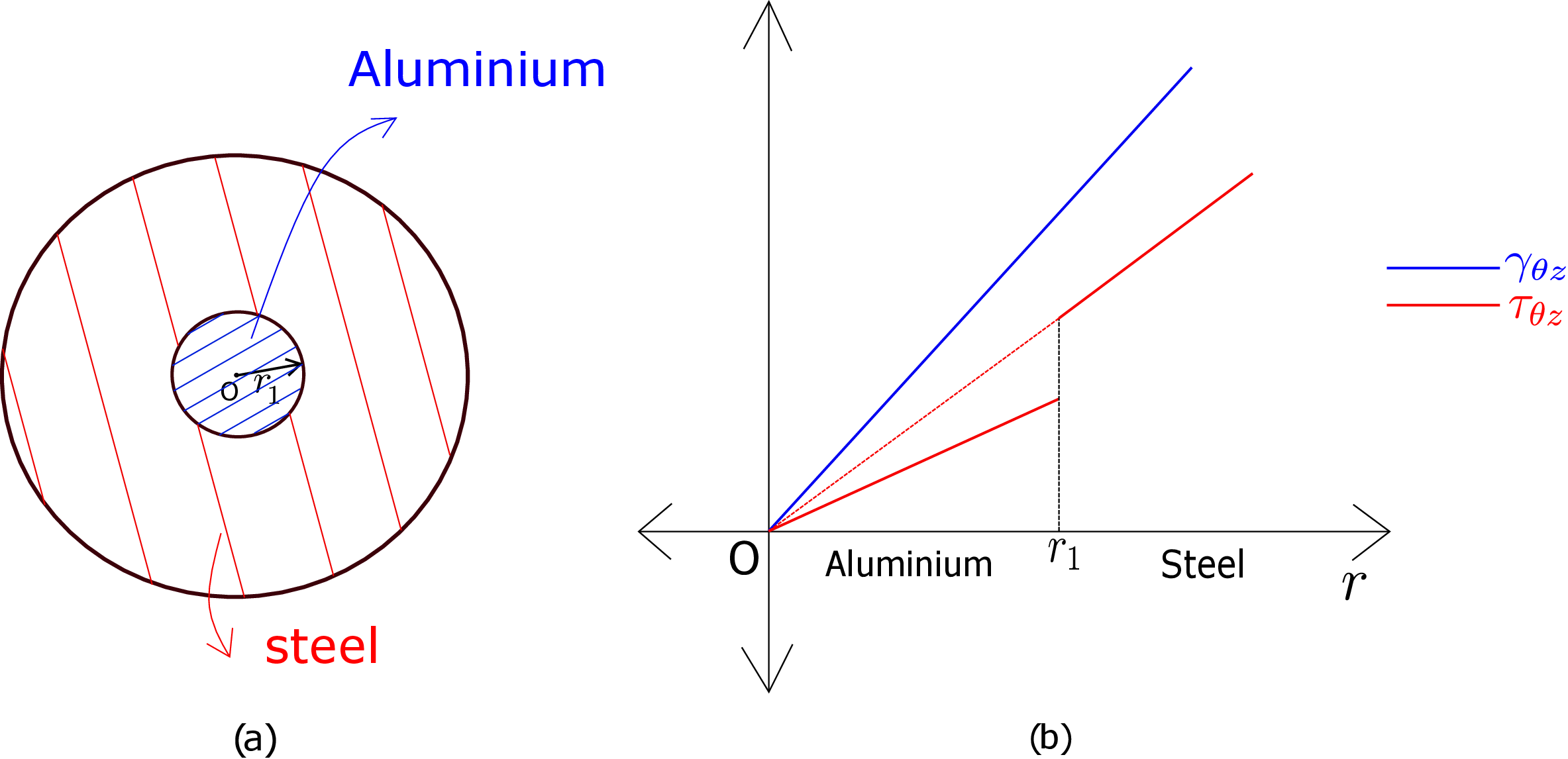
Supposing the inner part (up to radius \(r_1\)) is made up of Aluminium and the outer part is made up of Steel. The two parts are glued together or fitted tightly. If we now twist the composite cylinder, the cross section will again rotate as a whole. The shear strain \(\gamma _{\theta z}\) will then vary linearly in radius as earlier. However, when we calculate \(\tau _{\theta z}\) from equation \eqref{7_tau_theta_z}, we will have different shear modulus for aluminium and steel. Thus, there will be a discontinuity in shear stress at \(r=r_1\). The variation of \(\gamma _{\theta z}\) and \(\tau _{\theta z }\) for this cross-section is shown in Figure 7.24b. The variation of \(\gamma _{\theta z}\) is shown by the continuous blue line while the variation of \(\tau _{\theta z}\) is shown by the discontinuous red line which is piecewise linear: the slopes of the two parts are different and proportional to the shear modulus of the corresponding material. Working out the integration as in \eqref{7_torque} will give us the following formula for torque in a composite cylinder: \begin {equation} T = (G_A J_A + G_S J_S)\frac {\Omega }{L}. \end {equation} Here subscripts ‘\(A\)’ and ‘\(S\)’ denote aluminium and steel parts, respectively. One can think of an analogous relation relating axial force with axial strain for a composite cylinder.
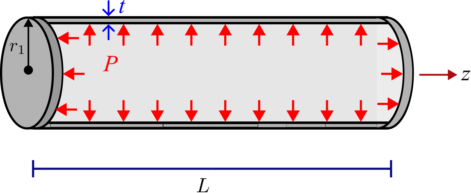
For pressurized thin cylinders which are capped at its two ends (see Figure 7.25), one can approximate the outer radius \(r_2\) to be almost equal to \(r_1\), i.e., \(r_2 \approx r_1\) and the thickness being \(t =r_2-r_1\). Using these, we arrive at the following simpler expressions of coefficients \(A\) and \(B\) (see equation \eqref{7_AB} above for exact expression): \begin {align*} A &= 2P \dfrac {r_1^2}{r_2^2 - r_1^2} = 2P \dfrac {r_1^2}{\brc {r_2+r_1}\brc {r_2-r_1}} \approx 2P \dfrac {r_1^2}{2 r_1 t} = \dfrac {P r_1}{t}, \\ B &= - P \dfrac {r_1^2 r_2^2}{r_2^2 - r_1^2} = -P \dfrac {r_1^2 r_2^2}{\brc {r_2+r_1}\brc {r_2-r_1}} \approx -P \dfrac {r_1^2 r_1^2}{2 r_1 t} = -\dfrac {P r_1^3}{2t}. \end {align*}
Now, substituting these values of \(A\) and \(B\) back in the expression for \(\sigma _{rr}\) and \(\sigma _{\theta \theta }\), and letting \(r \approx r_1\) we get: \begin {align*} \sigma _{rr} &= \dfrac {A}{2} + \dfrac {B}{r_1^2} = \dfrac {Pr_1}{2t} - \dfrac {P r_1^3}{2t r_1^2} = \dfrac {Pr_1}{2t} - \dfrac {P r_1}{2t } = 0,\\ \sigma _{\theta \theta } &= \dfrac {A}{2} - \dfrac {B}{r_1^2} = \dfrac {Pr_1}{2t} + \dfrac {P r_1^3}{2t r_1^2} = \dfrac {Pr_1}{2t} + \dfrac {P r_1}{2t} = \dfrac {P r_1}{t}. \end {align*}
To obtain thin tube approximation of \(\sigma _{zz}\), we saw earlier that \(\sigma _{zz}\) does not vary through the wall thickness. Accordingly when no external axial force acts on the cylinder, we have \begin {align*} \sigma _{zz} = \frac {\pi ~r_1^2~P}{\pi (r_2^2-r_1^2)}\approx \frac {Pr_1}{2t}. \end {align*}
Instead of deriving the thin-tube approximations from the formula of thick cylinders, we will now consider deriving them directly from force balance of various sections of a thin cylinder (see Figure 7.26).
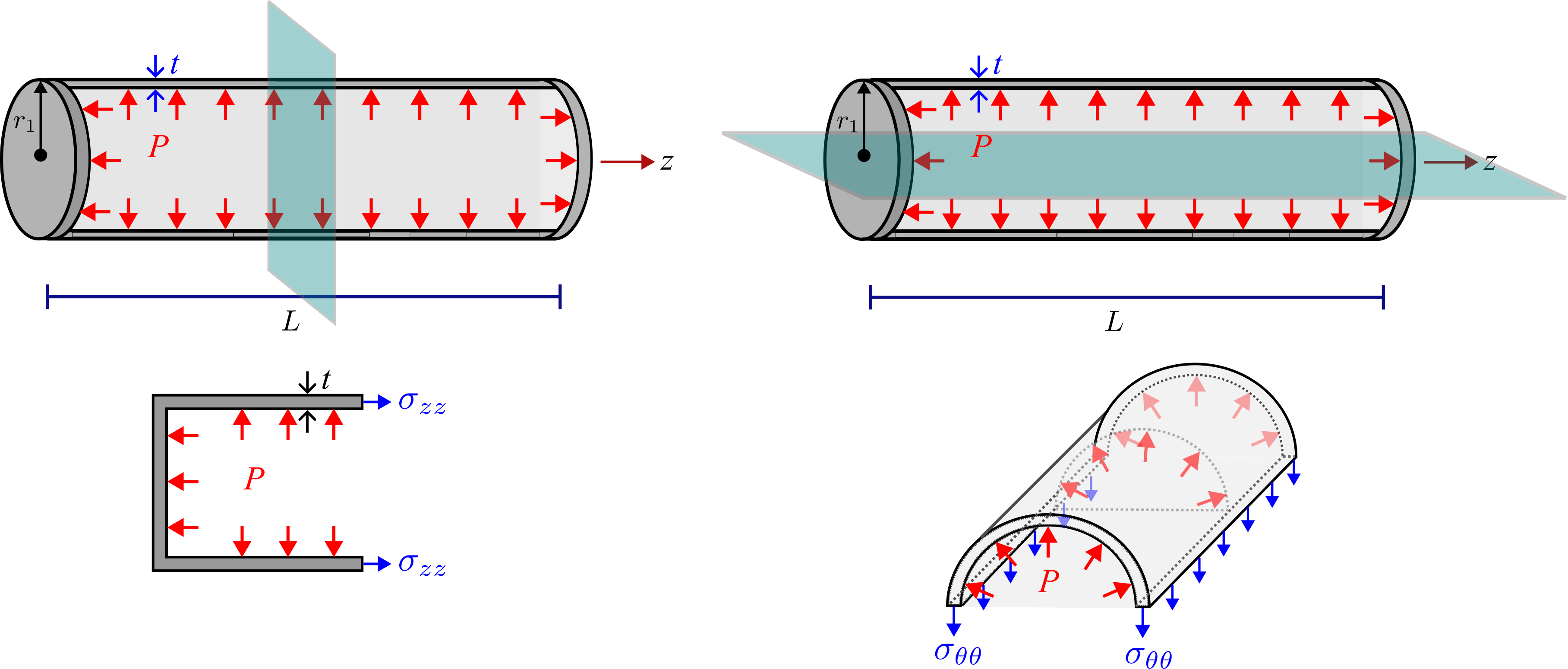
To obtain \(\sigma _{zz}\), we take a vertical section through the cylinder (see Figure 7.26a) and do force balance in \(z-\)direction, i.e., \begin {align*} \sigma _{zz} \brc {2 \pi r_1 t} = P \brc {\pi r_1^2}~\text {or}~ \sigma _{zz} = \dfrac {P r_1}{2t}. \end {align*}
To obtain \(\sigma _{\theta \theta }\), we take a horizontal section through the cylinder (see Figure 7.26b) and do force balance in vertical direction, i.e., \begin {align*} \sigma _{\theta \theta } \brc {2 L t} = P \brc {2 r_1 L}~\text {or}~ \sigma _{\theta \theta } = \dfrac {P r_1}{t}. \end {align*}
Note that pressure is thought of as acting over the projected area of \(2r_1L\).
To obtain radial stress \(\sigma _{rr}\), consider the outer traction-free surface (\(\sigma _{rr} = 0\)) and the internally pressurized surface (\(\sigma _{rr} = -P\)). Through
the thickness of thin tube, the radial stress drops sharply from \(-P\) at inner surface to zero at the outer surface.
However, \(\dfrac {r_1}{t} >> 1\) for thin tubes. Accordingly, the values of \(\dfrac {Pr_1}{t}\) and \(\dfrac {Pr_1}{2t}\) for hoop and axial stresses, respectively, will be very large
compared to \(P\). Accordingly, \(\sigma _{rr}\) is neglected and set to zero.
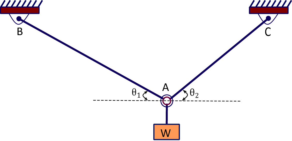
Solution: Using free body diagram and doing force balance, let us find tension in wires.
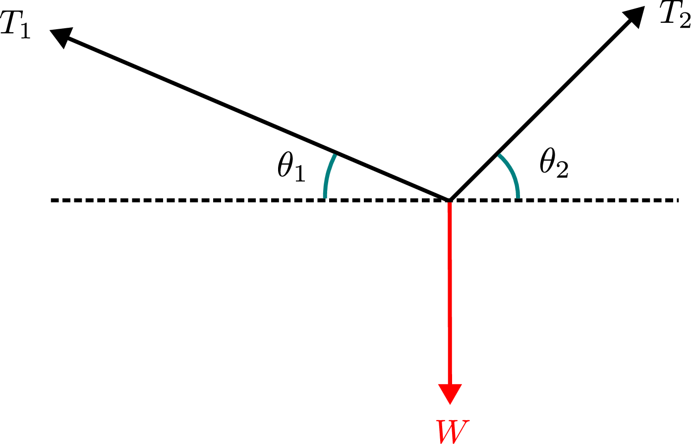
\begin {align*} \stackrel {+}\rightarrow \sum F_x \;=\;0\;\Rightarrow \; T_2 \cos \theta _2 \;-\;T_1 \cos \theta _1\;=\;0 \Rightarrow \; T_2\;=\;T_1 \dfrac {\cos \theta _1}{\cos \theta _2}. \end {align*}
\begin {align*} + \uparrow \;\sum F_y\;=\;0 &\Rightarrow \;T_1 \sin \theta _1 \;+\;T_2 \sin \theta _2 \;=\;W \Rightarrow T_1 \sin \theta _1 \;+\;T_1 \dfrac {\cos \theta _1}{\cos \theta _2} \sin \theta _2 \;=\; W\\ &\Rightarrow \; T_1 \;=\;\dfrac {W}{\cos \theta _1 \brc {\tan \theta _1 \;+\;\tan \theta _2}}~ \text {and} ~ \;T_2 \;=\;\dfrac {W}{\cos \theta _2 \brc {\tan \theta _1 \;+\;\tan \theta _2}}. \end {align*}
The stress in each wire should not exceed the prescribed limit, so check that \begin {align} \sigma _{1} \;=\;\dfrac {T_1}{A_1} \;=\;\dfrac {W}{A_1 \cos \theta _1 \brc {\tan \theta _1 \;+\;\tan \theta _2}} \;\le \; \sigma _{tol} \Rightarrow \; W\;\le \;\sigma _{tol}\sbk {A_1 \cos \theta _1 \brc {\tan \theta _1 \;+\; \tan \theta _2 } }, \label {7_1.1}\\ \sigma _{2}\;=\;\dfrac {T_2}{A_2}\;=\;\dfrac {W}{A_2\cos \theta _2 \brc { \tan \theta _1 \;+\;\tan \theta _2 }} \; \le \; \sigma _{tol} \Rightarrow \; W\; \le \; \sigma _{tol} \sbk { A_2 \cos \theta _2 \brc { \tan \theta _1 \;+\;\tan \theta _2 }}. \label {7_1.2} \end {align}
The maximum permissible load \(W\) would be the minimum of the loads obtained from relations \eqref{7_1.1} and \eqref{7_1.2}. Note that as the wires undergo extension, the angles \((\theta _1,\theta _2)\) would also change. However, we have assumed that such changes are negligible here.
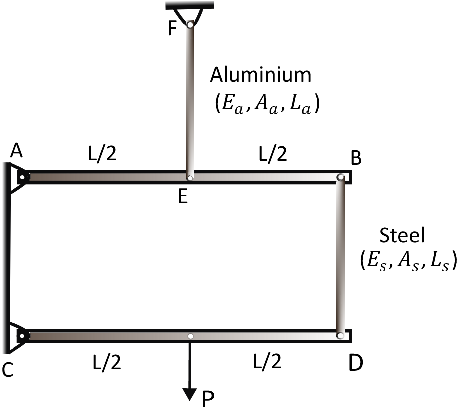
Solution: The bars AB and CD are rigid but the aluminium and steel rods are deformable. Let us first find the force acting in elements EF and BD to know how much they will stretch. To do that, we draw free diagrams and do force and moments balance of all the members. Note that all joints are pinned joints - hence no moment acts at these joints.
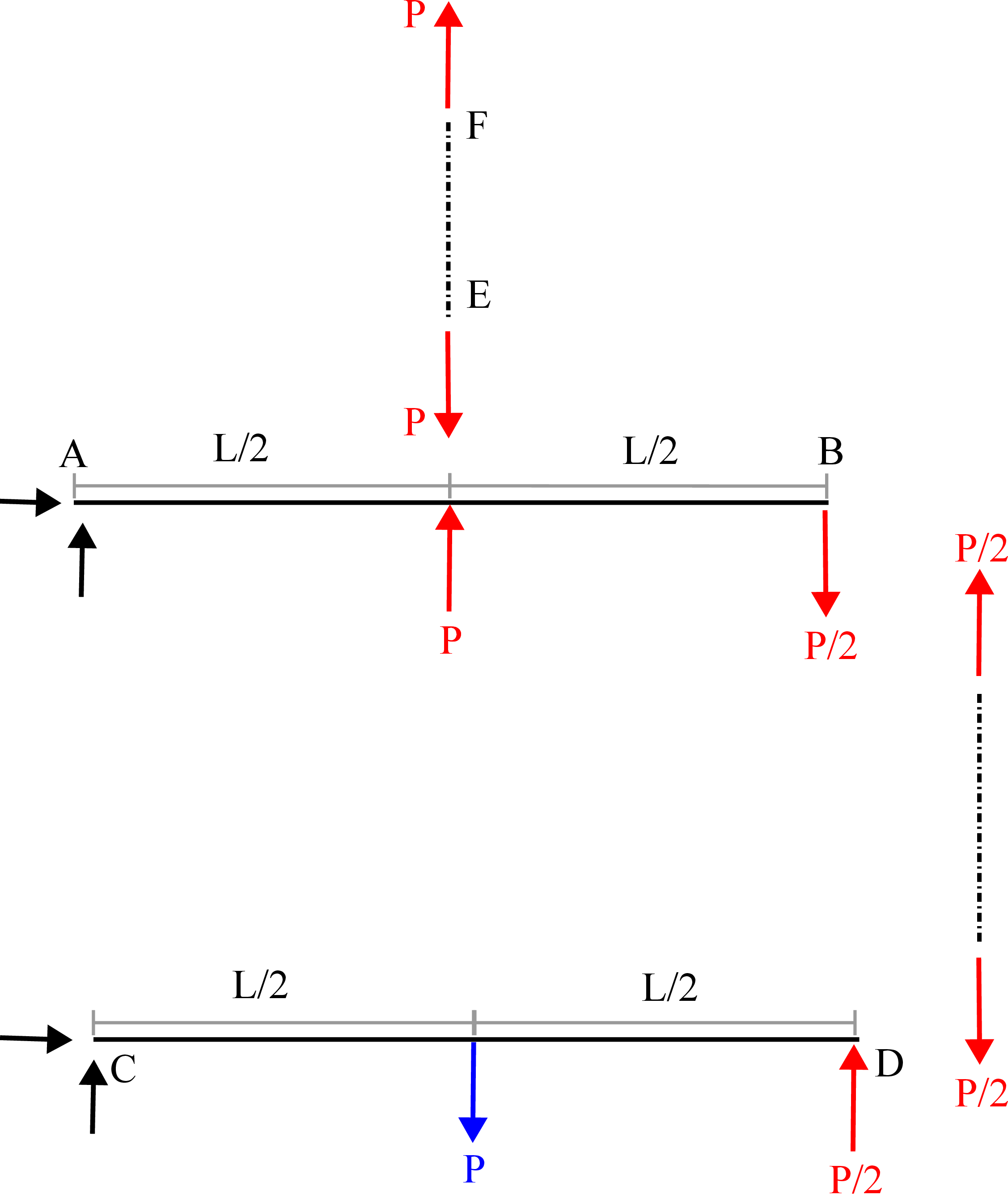
Aluminium rod EF: \begin {align*} \delta _{a}\;=\;\dfrac {Fl}{EA} \;=\;\dfrac {P L_{a}}{E_{a}A_{a}}. \end {align*}
This implies point \(E\) goes down by \(\delta _a\) whereas point \(B\) will accordingly go down by \(2\delta _a\). Steel rod BD: \begin {align*} \delta _s\;=\;\dfrac {Fl}{EA}\;=\;\dfrac {(P/2) L_s}{E_s A_s}. \end {align*}
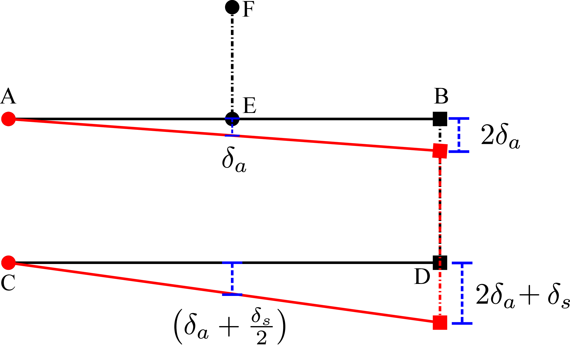
This implies point \(D\) goes down by \(2\delta _a+\delta _s\) and hence the the displacement of the point of application of load \(P\) turns out to be \begin {align*} \delta \;=\; \delta _{a} \;+\;\dfrac {\delta _s}{2} \; \le \;\delta _c \Rightarrow \; \dfrac {PL_{a}}{E_{a}A_{a}} \;+\;\dfrac {PL_s}{4 E_s A_s}\; \le \;\delta _c \quad \text {or}~ P\;\le \; \dfrac {\delta _c}{\dfrac {L_{Al}}{E_{Al}A_{Al}} \;+\;\dfrac {L_s}{4 E_s A_s }}. \end {align*}
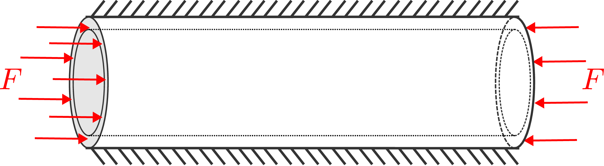
Solution: It might seem like a uniaxial loading problem. However, this is a biaxial loading problem since an unknown pressure will act on the outer lateral surface. The axial load causes the steel tube to compress axially and expand radially but the wall being rigid does not allow any radial expansion. So, in turn, the wall applies a compressive pressure on the outer surface of the tube. We can say that \(u_{\theta } = 0\), \(u_z \ne 0\), \(u_r \ne 0\). We need to find out \(\sigma _{\theta \theta }\). Let us first find out \(\sigma _{zz}\): \[\sigma _{zz} = \frac {F}{\frac {\pi (D^2-d^2)}{4}} = \frac {F}{\frac {\pi (D+d)(D-d)}{4}} = \frac {F}{\frac {\pi (d+2t+d)(2t)}{4}} = \frac {F}{\pi (d+t)t}.\] Here we used the fact that \(\sigma _{zz}\) does not vary through the wall thickness as proved in the theory. The solution of \(\sigma _{rr}\) and \(\sigma _{\theta \theta }\) from radial stress equilibrium equation in cylindrical coordinates are as follows: \begin {align*} \sigma _{rr}\;=\;\dfrac {A}{2}\;+\;\dfrac {B}{r^2}, \quad \sigma _{\theta \theta } \;=\;\dfrac {A}{2}\;-\;\dfrac {B}{r^2}. \end {align*}
The values of integrating constants \(A\) and \(B\) can be obtained using boundary conditions!
Traction BC: No internal pressure: \begin {align*} &\Rightarrow \sigma _{rr}\brc {r_1}\;=\;0 \\ &\text {We can't say }\sigma _{rr}\brc {r_2}\;=\;0 \text { since the outer constraining pressure is an unknown.} \end {align*}
Displacement BC: No radial displacement at the outer boundary: \begin {align*} u_r\brc {r_2}\;=\;0. \end {align*}
The radial displacement \(u_r\) is given by \(u_r = \frac {Cr}{2} + \frac {D}{r}\) and the integrating constants \(A\) and \(B\) in the radial stress expression above are related to \(C\) and \(D\) as follows: \begin {align*} A = (\lambda + \mu ) C + \lambda u_z^{'}, \quad B = 2\mu D. \end {align*}
We also have \(u_z'=1/E(\sigma _{zz}-\nu (\sigma _{rr}+\sigma _{\theta \theta }))=1/E(\sigma _{zz}-\nu ~A)\) which when substituted in the above equation leads to \begin {align*} C=1/(\lambda +\mu )\left [A(1+\lambda \nu /E)-\lambda /E~\sigma _{zz}\right ],~D=B/2\mu . \end {align*}
So, the final equations to obtain \(A\) and \(B\) are \begin {align*} &\sigma _{rr}(r_1)=0\Rightarrow \frac {A}{2}+\frac {B}{r_1^2} = 0,\nonumber \\ &u_r(r_2)=0\Rightarrow A\frac {1+\lambda \nu /E}{2(\lambda +\mu )}r_2 + \frac {B}{2\mu r_2} - \nu /E~\frac {F}{\pi (d+t)t}r_2=0. \end {align*}
One can then also evaluate \(\sigma _{rr}(r_2)\) to obtain the unknown pressure applied by the rigid hole.
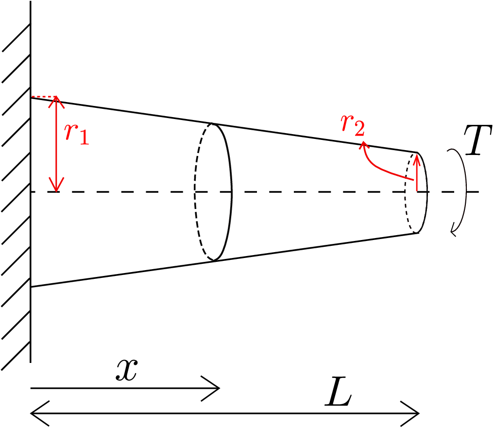
Solution: We had derived the end-to-end rotation \(\Omega \) to be \begin {equation} \label {7_end_end_rotation} \Omega =\frac {TL}{GJ} \end {equation} but it holds only when the cross-section is uniform over the entire length. For the current case, a different form of the above equation is useful as shown below: \begin {equation} \label {torque_twist_relation} T=GJ\underbrace {\bigg (\frac {\Omega }{L}\bigg )}_{\text {twist($\kappa $)}}=GJ\kappa \end {equation} where \(\kappa \) denotes twist or the rate of change of rotation of the cross section. As the same torque \(T\) acts in every cross-section (as shown below), the above equation implies that twist varies along the length as the polar moment of area \(J\) is varying here due to varying radius. For an even general case where the material of the tube as well as torque changes along the length, one can use the below formula to obtain twist at a given location: \begin {equation} \label {7_torque_relation_at_x} T(x)=G(x)J(x)\kappa (x) \end {equation} where the twist \(\kappa \) is related to cross-sectional rotation \(\Omega \) through \begin {equation} \kappa (x)=\frac {d\Omega }{dx}.\notag \end {equation}
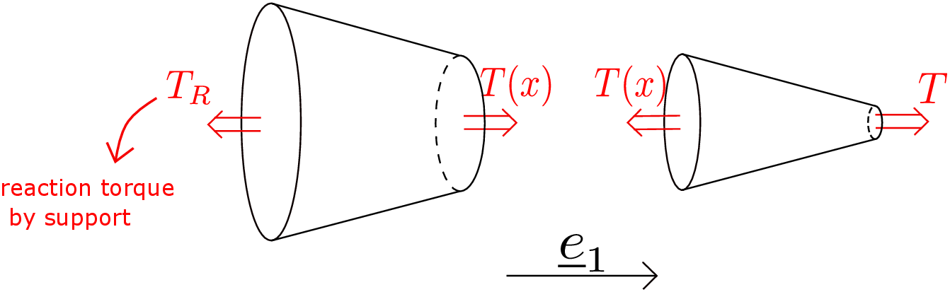
The variation of \(T\) along the axis of the cylinder can be found by making a free body diagram. We cut a section of the cylinder at a distance \(x\) from the clamped end. The two cut parts are shown in Figure 7.27. The external torque \(T\) acts on the right end of the right part.††† There will be an internal torque on the other end of the right part. As this cross-section has its normal along \(-\underline {e}_1\), the torque \(T(x)\) will act here in \(-\underline {e}_1\) direction. Similarly, as the cross-section normal of the right end of the left part points in \(+\underline {e}_1\) direction, the torque on it points along \(+\underline {e}_1\) direction. We then do moment balance for the right part leading to
This means that the torque at every cross-section is the same and equal to the applied external torque \(T\) even though the cross-sectional radius is changing. Assuming that the cylinder is made up of a single material, its shear modulus will also be a constant. To find \(J(x)\) for a cross-section of radius \(r(x)\), we integrate over the area of the cross section, i.e.,
We thus obtain
The end-to-end rotation then becomes
As \(r\) varies linearly along the axis of the cylinder and
the radius for a general cross-section can be found by linear interpolation of the above two points, i.e., \begin {equation} r(x)=r_1+\frac {r_2-r_1}{L}x.\notag \end {equation} We can substitute this in equation \eqref{7_rotation_in_terms_of_r_x} to get \begin {equation} \Omega (L)=\frac {2T}{\pi G}\int _0^L\frac {1}{\big (r_1+\frac {r_2-r_1}{L}x\big )^4}dx. \end {equation}
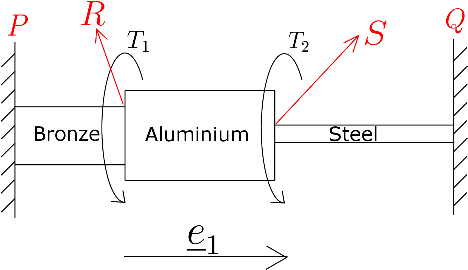
Solution: We first need to find the torque acting on each of the three parts of the shaft. Figure 7.28 shows the free body diagram of the entire shaft.
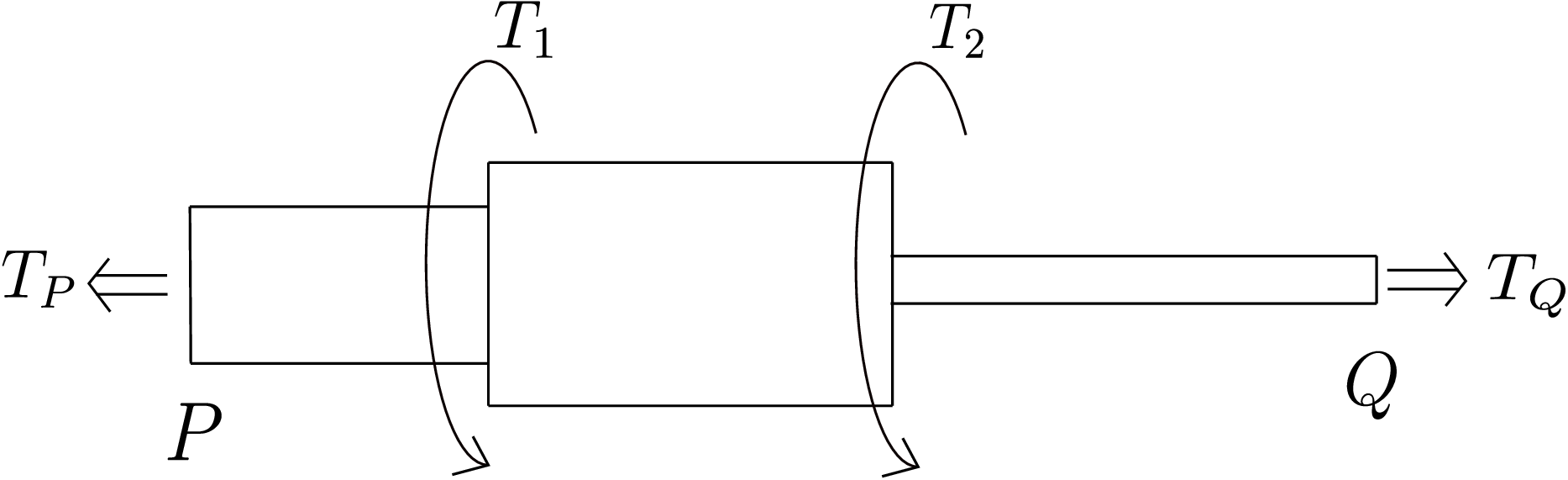
The torques \(T_1\) and \(T_2\) are externally applied torques and point in the \(\underline {e}_1\) direction while \(T_P\) and \(T_Q\) are reaction torques applied by the clamped supports. The torque \(T_P\) is shown pointing in negative direction because the cross section normal at \(P\) points along \(-\underline {e}_1\) direction. The moment balance of the entire shaft gives us \begin {equation} T_Q~\underline {e}_1+(T_1+T_2)~\underline {e}_1-T_P~\underline {e}_1=0\nonumber \end {equation} \begin {equation} \Rightarrow \boxed {T_Q-T_P+T_1+T_2=0}\notag \end {equation} As there are no forces acting on the shaft, force balance will not give us anything. So, we have one equation and two unknowns \(T_P\) and \(T_Q\). Thus, this is a statically indeterminate problem. To solve such problems, we need to take deformation into account. The strain matrix due to torsion will be \begin {equation} \begin {bmatrix} \underline {\underline {\epsilon }} \end {bmatrix}_{(r,\theta ,z)}= \begin {bmatrix} 0 & 0 & 0\\ 0 & 0 & \dfrac {\kappa r}{2}\\ 0 & \dfrac {\kappa r}{2} & 0 \end {bmatrix}.\notag \end {equation} where \(\kappa \) denotes twist. The stress matrix then becomes \begin {equation} \label {7_torsion_state_of_stress} \begin {bmatrix} \underline {\underline {\sigma }} \end {bmatrix}_{(r,\theta ,z)}= \begin {bmatrix} 0 & 0 & 0\\ 0 & 0 & G\kappa r\\ 0 & G\kappa r & 0 \end {bmatrix}. \end {equation} It is the state of stress at any point in the composite shaft. At a point, we have infinite planes. We need the plane on which the shear component of traction is maximum. In the chapter on Mohr’s circle, we had discussed that for finding the maximum shear component, we need to obtain the difference of the maximum and minimum principal stresses and divide that by 2. To find the principal stress components, we can use the concept of Mohr’s circle. As the first column of the stress matrix is all zero, \(\underline {e}_r\) is a principal axis. Thus, we can draw the Mohr’s circle for those planes whose normals are of the form: \begin {equation} \underline {n}=\cos \theta \,\underline {e}_\theta +\sin \theta \,\underline {e}_z.\notag \end {equation} The center of the circle will be at the mid point of \(\sigma _{\theta \theta }\) and \(\sigma _{zz}\) on \(\sigma \)-axis. As both of them are zero, the center will be at origin. We then mark the value of \(\tau _{\theta z}\) (\(=G\kappa r\)) on \(\tau \)-axis. This point corresponds to \(\theta \)-plane. With center and \(\theta \) plane known, we get the radius by joining these two points which equals \(G\kappa r\). The Mohr’s circle so obtained is shown in Figure 7.29.
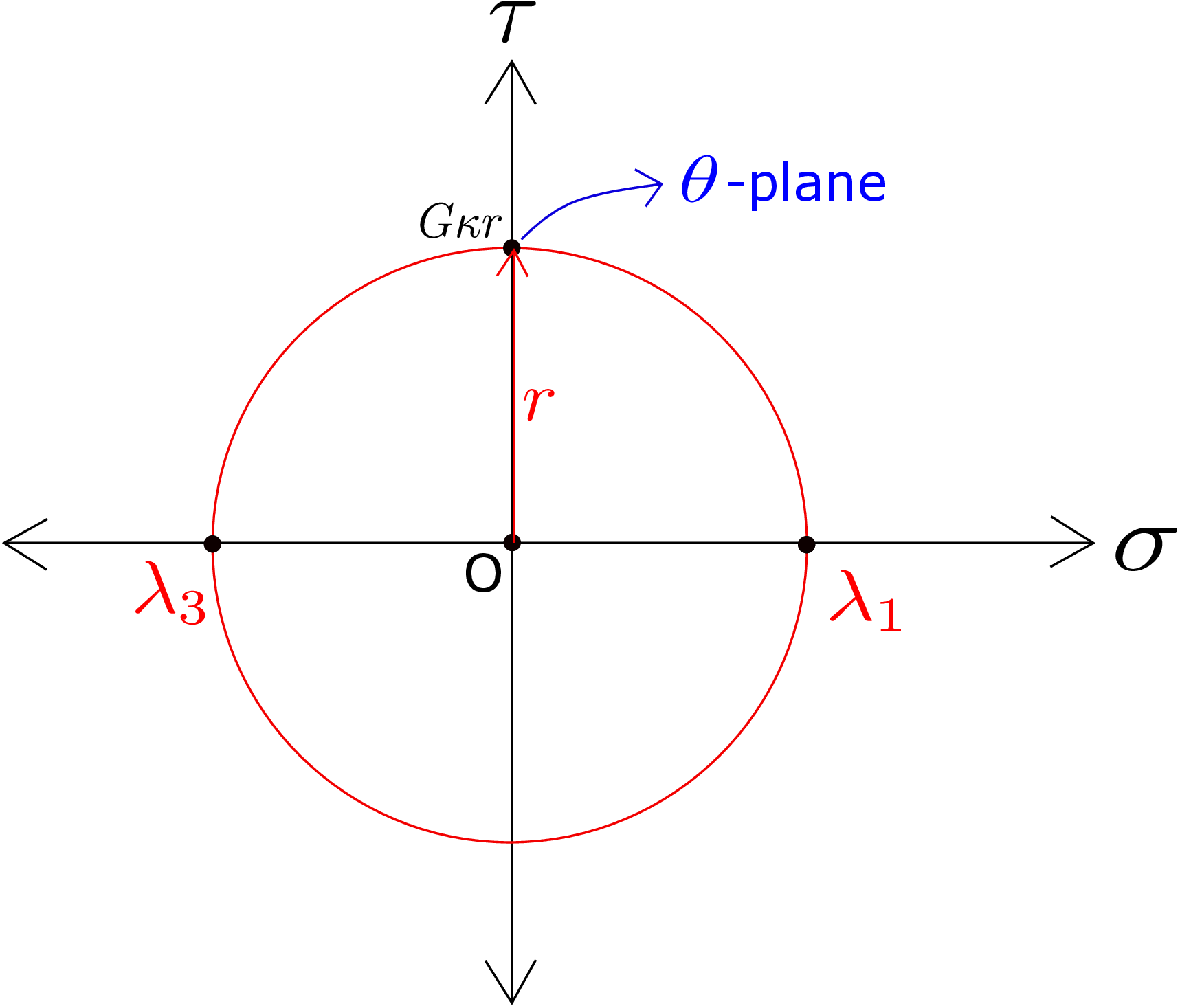
We can now extract the principal stress components from the circle, i.e.,
and \(\lambda _2\) is zero corresponding to \(\underline {e}_r\) principal direction. The maximum shear component of traction is thus
We have to find the maximum shear component of traction for each of the three sub-shafts. From our above analysis, it turns out to be \(G\kappa r\) and \(r\) is maximized for points on the lateral surface. We also need to find the value of twist for each of the three shafts. We had found in the previous problem (equation \eqref{7_torque_relation_at_x}) that torque at an arbitrary cross section is given by \begin {equation} T(z)=G(z)\kappa (z)J(z). \end {equation} The twist \(\kappa \) is then \begin {equation} \label {7_kappa_at_z} \kappa (z)=\frac {T(z)}{G(z)J(z)}. \end {equation} As each sub-shaft is made up of a single material and has a constant cross section radius, the denominator \(G(z)J(z)\) is constant for the three sub-shafts separately. We just need to find the variation of torque in each of them. We first draw the free body diagram of a part of the bronze shaft. We make a cut in the bronze shaft and consider its left part as shown in Figure 7.30.
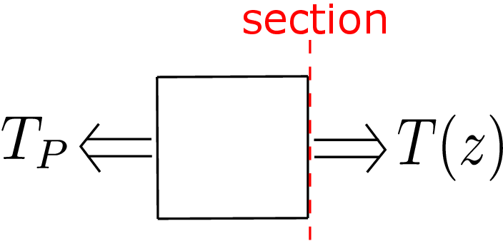
\(T_P\) acts as a reaction torque from the left support and \(T(z)\) is exerted by the other part of bronze shaft. Balance of moment then gives \begin {equation} \label {7_torque_bronze} T_B=T_P \end {equation} where \(T_B\) represents the torque within the bronze shaft and it does not vary within the bronze shaft. Now, we cut a section in the aluminium shaft such that bronze and aluminium shafts are included in the left part and draw its free body diagram (see Figure 7.31).
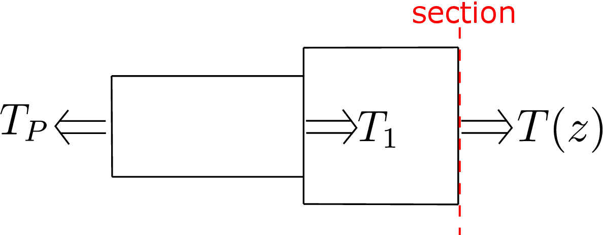
This time we also have external torque \(T_1\) acting in the free body diagram. Moment balance gives torque in the Aluminium section (\(T_{A}\)) as \begin {equation} \label {7_torque_aluminium} T_{A}=T_P-T_1. \end {equation} Finally, we cut a section in the steel shaft such that all three materials are included in the left part. We draw the free body diagram of this left part as shown in Figure 7.32.
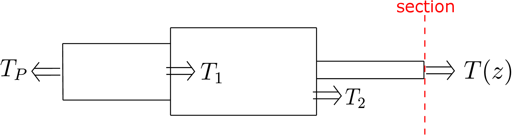
Moment balance gives torque in the steel section (\(T_S\)) as \begin {equation} \label {7_torque_steel} T_S=T_P-T_1-T_2. \end {equation} We can see that torque within each of the three shafts does not vary. But, we can also observe that \begin {equation} T_B\neq T_{A}\neq T_S. \end {equation} If we now come back to equation \eqref{7_kappa_at_z}, all the quantities on the RHS are constants within each sub-shaft separately. Thus, the twist \(\kappa \) is also a constant within each of the three sub-shafts. At the same time, its value is different for the three sub-shafts as their radii, \(G\) and \(T\) values are distinct. To find the maximum shear component of traction (\(=G\kappa r\)), we need the value of twist in the three regions. We have expressed the torques in the three sub-shafts in terms of \(T_P\) which is still an unknown. To find this unknown \(T_P\), we need to use the constraint that the two ends of the shaft are clamped. So, both the ends do not undergo any rotation and the end-to-end rotation for the composite shaft must be zero. Thus, the sum of the end-to-end rotations for the three sub-shafts should be zero. This is the extra equation that required taking deformation into account. Using equation \eqref{7_end_end_rotation}, the end-to-end rotations for each of the sub-shafts will be
Adding the three equations , we finally get
However, \(\Omega _Q-\Omega _P\) is zero since, being clamped, \(\Omega _Q\) and \(\Omega _P\) are individually zero. We can now substitute \(T_B\), \(T_A\) and \(T_S\) from equations \eqref{7_torque_bronze}, \eqref{7_torque_aluminium} and \eqref{7_torque_steel} into \eqref{7_end-to-end} to obtain
This equation is solved for \(T_P\). Once we get \(T_P\), we can find torque in the three sub-shafts from equations \eqref{7_torque_bronze}, \eqref{7_torque_aluminium} and \eqref{7_torque_steel} and hence twist in them using equation \eqref{7_kappa_at_z}. Then, we can use equation \eqref{7_tau_max} to calculate the max shear component of traction in the three sub-shafts. Remember to use the outer radius of the three sub-shafts to obtain the maximum shear component.
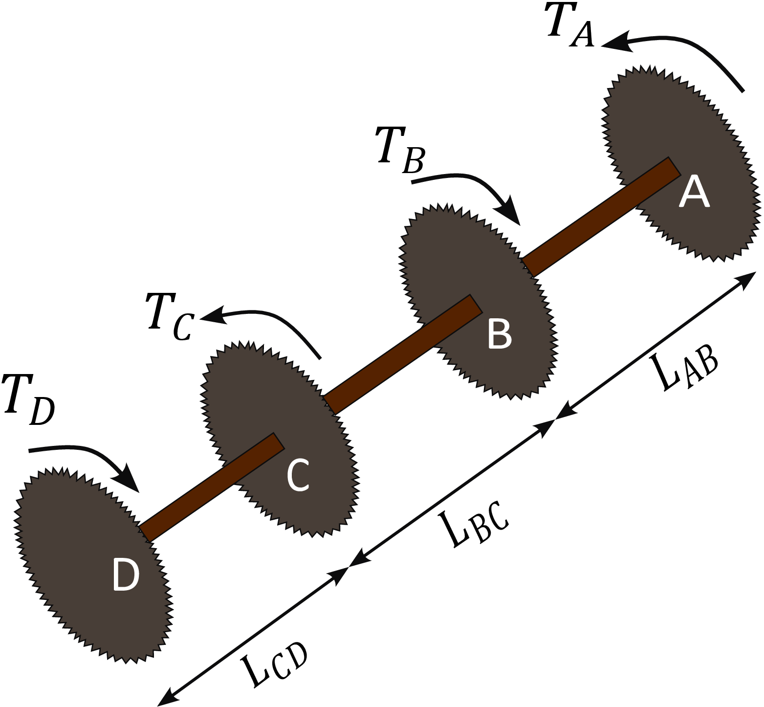
Solution: As the net torque \(T_A + T_B + T_C + T_D\) is zero, it is a static problem. Let us assume the \(+\ve {e}_3\) axis to be pointing from D towards A. Accordingly, positive/negative torques are determined by the right-hand-thumb rule with the thumb pointing along \(+\ve {e}_3\) direction. To determine the relative rotation of point A w.r.t. point D, we need to determine relative rotation of individual segments AB, BC, and CD using the formula \[\Omega = \frac {T L}{G J}.\] The torques in each segment is different here though which can be determined from the below torque diagram - it depicts variation in torque along the shaft.
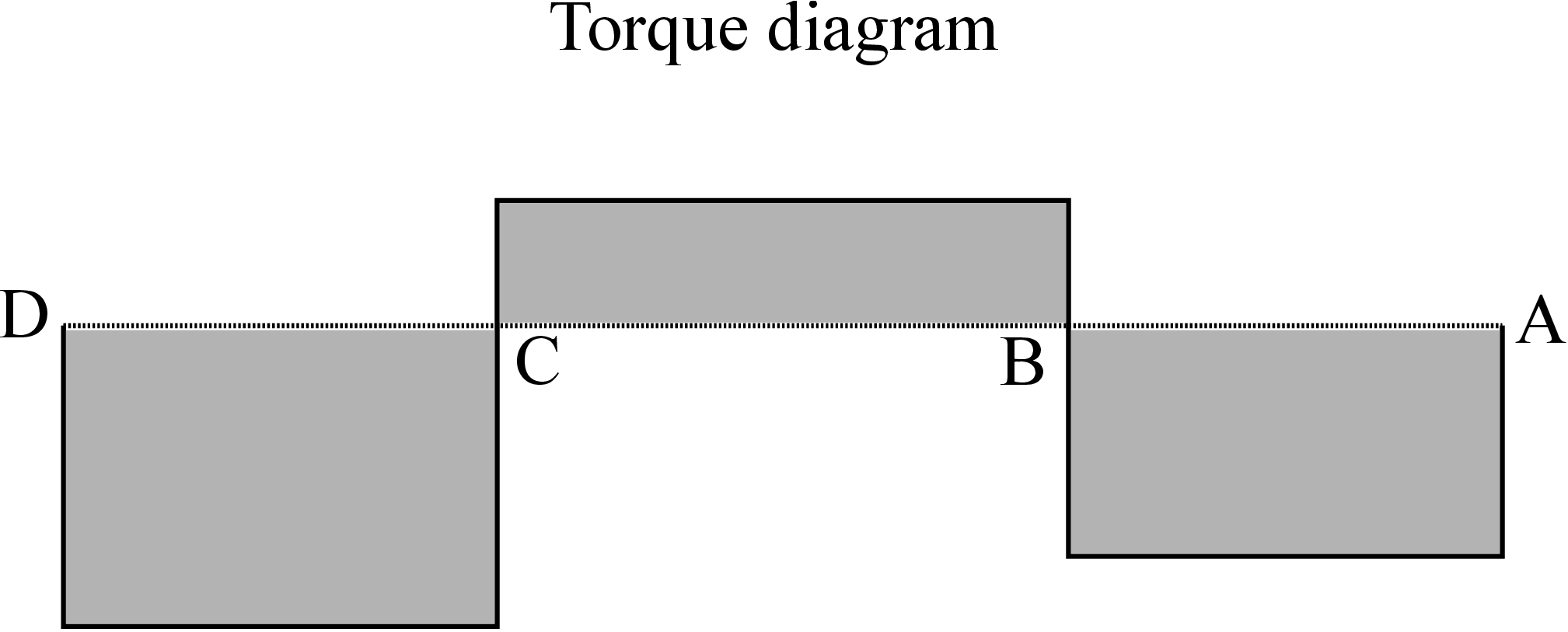
We have assumed here that \(T_B>T_A\). Basically \[T_{AB}=-T_A,~T_{BC}=T_B-T_A, T_{C_D}=T_B-T_A-T_C=-T_D.\] If \(\Omega _{AD}\) is the relative rotation of point A w.r.t. point D, then \begin {align*} \Omega _{AD} &= \Omega _{AB} + \Omega _{BC} + \Omega _{CD}= \frac {T_{AB} L_{AB} + T_{BC} L_{BC} + T_{CD} L_{CD}}{G J}. \end {align*}
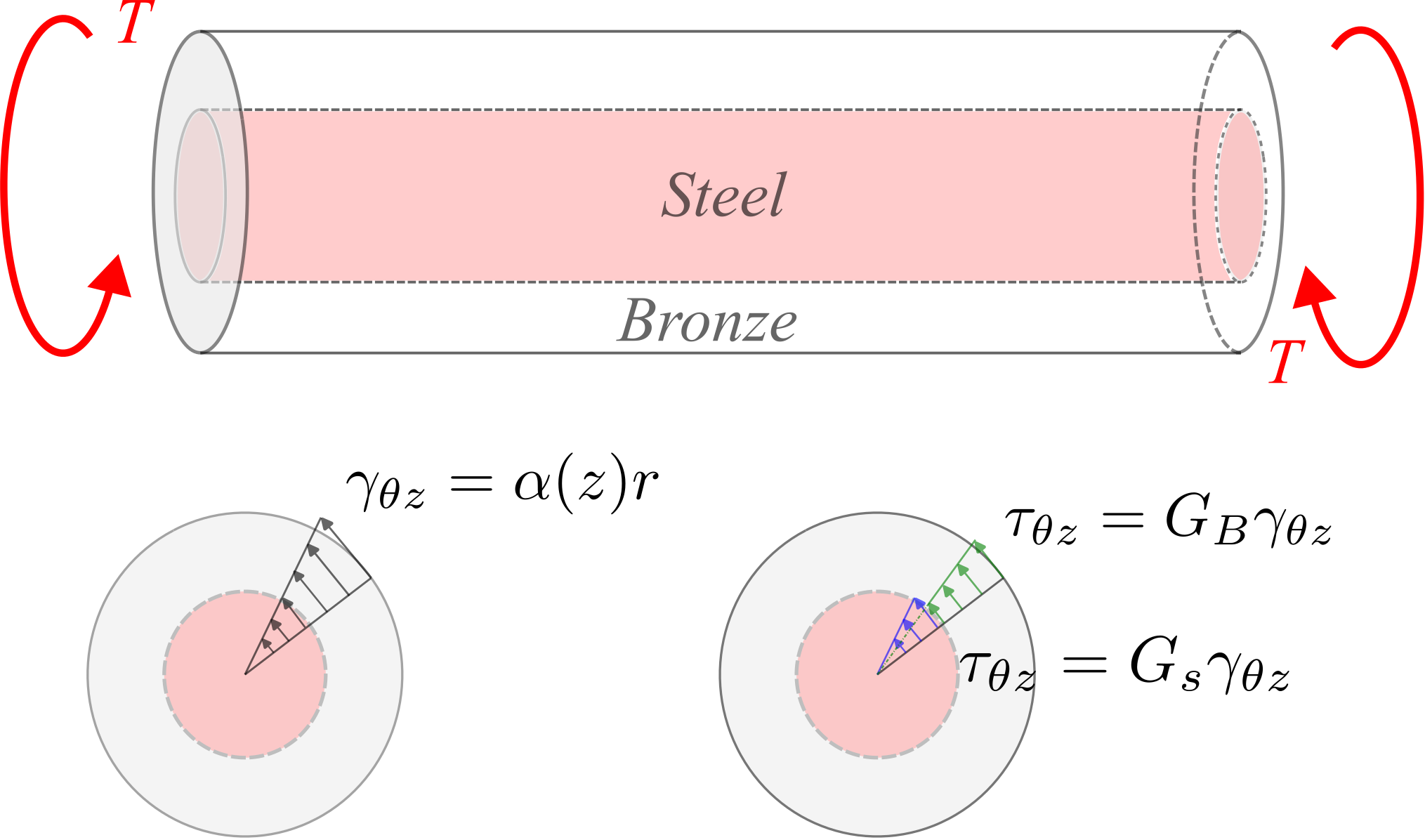
Solution: The shear strain \(\gamma _{\theta z}\) varies linearly with \(r\) in both the materials since the two parts are fastened together rigidly and hence the twist value \(\kappa \) would be the same in the two materials. The shear stress \(\tau _{\theta z}\) is proportional to shear strain but shear modulus being different for two materials, it will exhibit a jump across the interface for the two materials - see figure above. Accordingly, total torque in the cross-section equals \begin {align*} \int \int \tau _{\theta z} ~dA &= \int \int _{Steel} G_S ~\kappa ~ r^2 dA+ \int \int _{Bronze} G_B ~\kappa ~ r^2 dA=G_S J_S ~\kappa + G_B J_B~ \kappa \\ \Rightarrow T\;&=\;T_S\;+\;T_B. \end {align*}
As the twist \(\kappa \) is the same across the cross-section, the torques \(T_S\) and \(T_B\) obey \begin {align*} &\dfrac {T_S}{G_S J_S}\;=\;\dfrac {T_B}{G_B J_B} \Rightarrow T_S\;=\;T_B \brc {\dfrac {G_S J_S}{G_S J_B}}\\ &\text {or}~ T\;=\;T_S\;+\;T_B\;=\;T_B\brc {\dfrac {G_S J_S}{G_B J_B}}\;+\;T_B\;=\;T_B\dfrac {\brc {G_S J_S\;+\;G_B J_B} }{G_B J_B}\\ &\text {or}~ T\;=\;T_S\;+\;T_B\;=\;T_S\;+\;T_S\brc {\dfrac {G_B J_B}{G_S J_S}}\;=\;T_S\dfrac {\brc {G_S J_S\;+\;G_B J_B} }{G_S J_S} \end {align*}
Here \(J_S\;=\;\pi d^4/32\) and \(J_B\;=\;\pi \brc {D^4\;-\;d^4}/32\). Next we need to check for the maximum shear stress in each of the parts:
Steel \begin {align*} \tau _{S,max}\;=\;\dfrac {T_S r_S}{J_s}\;=\;\dfrac {T_S d}{2 J_S}\;\leq \;\tau _{S,tol}\Rightarrow T_S\;\leq \;\tau _{S,tol} \dfrac {2 J_S}{d}. \end {align*}
Bronze \begin {align*} \tau _{B,max}\;=\;\dfrac { T_B r_B}{J_B}\;=\; \dfrac {T_B D}{2 J_B }\;\leq \;\tau _{B,tol} \Rightarrow \; T_B\;\leq \; \tau _{B,tol}\dfrac {2 J_B}{D}. \end {align*}
\[\text {Hence}~T\;=\;\min \cbk {\tau _{B,tol}\dfrac {2 J_B}{D}\dfrac {\brc {G_S J_S \;+\;G_B J_B} }{G_B J_B}, \;\tau _{S,tol} \dfrac {2 J_S}{d} \dfrac {\brc {G_S J_S \;+\;G_B J_B} }{G_S J_S} }.\]
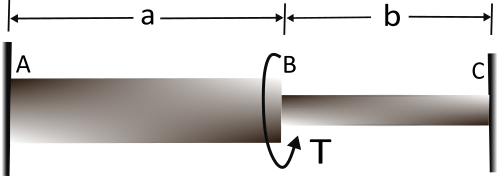
Solution: Let the end reaction torques be \(T_L\) and \(T_R\), respectively, at left and right fixed ends as shown in the figure below.
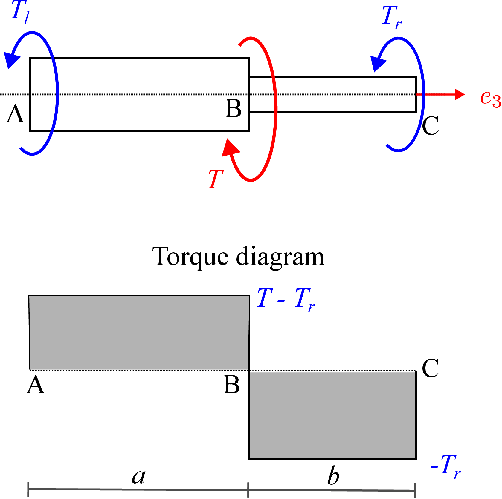
The two reaction torques are unknowns. Let us use moment balance of the full beam about its axis: \begin {align*} -T_R\;+\;T\;-\;T_L\;=\;0 \quad \text {or}~ \;T\;=\;T_R\;+\;T_L \end {align*}
which gives us one equation. It turns out we do not get any further equation from statics to obtain the two reaction torques. Hence, it is also a statically indeterminate problem. We need to use torque-twist relation to obtain the two reaction torques which we now show. Let
\(\Omega _{BC}\;=\) rotation of end C w.r.t end B,
\(\Omega _{AB}\;=\) rotation of end B w.r.t end A,
\(\Omega _{AC}\;=\) rotation of end C w.r.t end A.
Since the two ends are fixed, no rotations are allowed at A and C. Therefore \(\Omega _{AC}\;=\;0\). However \begin {align*} &\Omega _{AC}\;=\;\Omega _{AB}\;+\;\Omega _{BC}\\ \Rightarrow \;&\Omega _{AB}\;=\;-\Omega _{BC} \Rightarrow \;\dfrac {T_{AB}L_{AB}}{ G_{AB} J_{AB} }\;=\;-\dfrac {T_{BC}L_{BC}}{G_{BC} J_{BC}}\quad \text {or}~ \;\dfrac {T_L a}{G_B J_B}\;=\;\dfrac {T_R b}{ G_S J_S}. \end {align*}
So, \begin {align} T_L\;=\;T_R\brc {\dfrac {b}{a}}\brc {\dfrac {G_B J_B}{G_S J_S}} ~\text {or}~T_R\;=\;T_L \brc {\dfrac {a}{b}} \brc {\dfrac {G_S J_S}{G_B J_B}}.\notag \end {align}
So, total torque \begin {align} T\;=\;T_L\;+\;T_R =\;T_L\brc {\dfrac {G_B J_Bb\;+\;G_S J_S a}{G_B J_B b}}~ \text {or}~T\;=\;T_R\brc {\dfrac {G_B J_Bb\;+\;G_S J_S a}{G_S J_S a}}\label {eq:2b} \end {align}
Check for bronze (\(\tau _{max,B }\;\leq \;\tau _{tol,B} \)) \begin {align*} \tau _{max,B}\;=\dfrac {T_L~ r_B}{J_B} \Rightarrow \;T_L\;\le \;\dfrac {\tau _{tol,B} J_B}{r_B} \end {align*}
So, using eq. \eqref{eq:2b}, total torque \[T\;\le \;\brc {\dfrac {\tau _{tol,B}~J_B}{r_B}}\brc {\dfrac {G_B J_B b\;+\;G_S J_S a}{G_B J_B b}} \] Check for steel (\(\tau _{max,S}\;\leq \;\tau _{tol,S}\) ) \begin {align*} \tau _{max,S}\;=\;\dfrac {T_R~ r_S}{J_S}\Rightarrow \; T_R\;\le \;\dfrac {\tau _{tol,S} J_S}{r_S} \end {align*}
Again, using eq. \eqref{eq:2b}, total torque \[T\;\le \;\brc {\dfrac {\tau _{tol,S}~J_S}{r_S}}\brc {\dfrac {G_B J_B b\;+\;G_S J_S a}{G_S J_S a}}\] Maximum permissible torque T will be the minimum of above two values.
Solution:
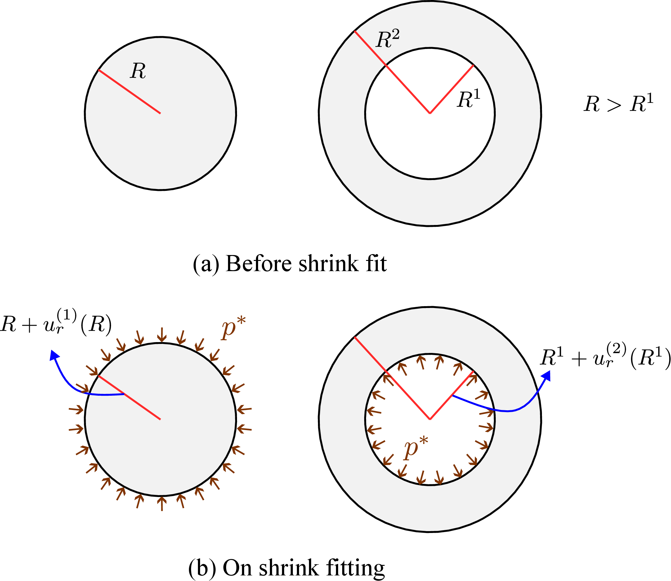
Shrink-fit insertion is usually performed by heat treatment, i.e., by heating the hollow disc (thereby expanding its
diameter), fitting it over the solid disc and then cooling it. You could imagine that shrink-fitting results in generation
of an interface pressure \(p^*\) over the external surface of the solid disk or over the inner surface of the hollow disk, as
required to eliminate the overlap \(R-R^1\).
We denote the solid disc and the hollow disc by superscripts \((1)\) and \((2)\) respectively. For example, \(\sigma ^{(1)}_{rr}\) and \(\sigma ^{(2)}_{rr}\) represent radial
stress in solid and hollow discs, respectively. For the problem at hand, the discs will only undergo
displacement in radial direction, i.e. \(u_{\theta } = u_z = 0\). As no body force acts, the radial equation when solved leads to
\begin {align*} \sigma _{rr}^{(1)}(r) = A^{(1)}/2+B^{(1)}/r^2,\quad \sigma _{rr}^{(2)}(r) = A^{(2)}/2+B^{(2)}/r^2 \end {align*}
or, in terms of radial displacement, we have \begin {align*} u_{r}^{(1)}(r) = C^{(1)}r/2+D^{(1)}/r,\quad u_{r}^{(2)}(r) = C^{(2)}r/2+D^{(2)}/r. \end {align*}
For the current problem where axial strain \(\epsilon =0\), we had derived \begin {align*} A^{(i)}=2(\lambda +\mu )C^{(i)}, \quad B^{(i)} = -2\mu ~D^{(i)}. \end {align*}
We have basically four independent integrating constants which will require four boundary conditions as mentioned
below:
(a) Boundary conditions: \begin {align*} &\sigma ^{(1)}_{rr}\brc {R}\;=\;\sigma ^{(2)}_{rr}\brc {R^1} \text { (continuity of radial stress)}\\ &R + u_r^{(1)}\brc {R} \;=\; R^1 + u_r^{(2)}\brc {R^1} \text { (shrink-fitting condition)}\\ &\sigma ^{(2)}_{rr}\brc {R^2}\;=\;0 \text { (traction-free boundary condition)}\\ &\sigma ^{(1)}_{rr}\brc {0}\;=\;\text {finite!} \quad \text {or}~ u_r^{(1)}(0) = 0. \end {align*}
Note that radial stress is continuous at the interface. The same cannot be said about hoop stress.
In fact, only the three traction components on radial plane will be continuous across the interface
because they form action-reaction pairs on the two radial faces of solid and hollow cylinders at the
interface.
(b) In terms of the unknown constants appearing in the displacement formula above, we can write the following for
radial stress: \begin {align*} \sigma _{rr}^{(1)}(r) = (\lambda +\mu )C^{(1)}-2\mu ~D^{(1)}/r^2,\quad \sigma _{rr}^{(2)}(r) = (\lambda +\mu )C^{(2)}-2\mu ~D^{(2)}/r^2. \end {align*}
Next, we apply the boundary conditions to determine the four integrating constants.
Using \(\sigma ^{(1)}_{rr}\brc {0}=\) finite \(\Rightarrow D^{(1)}=0\). \begin {align} &\text {Applying first boundary condition: } \sigma ^{(1)}_{rr}\brc {R}\;=\;\sigma ^{(2)}_{rr}\brc {R^1} \notag \\ &\Rightarrow \brc {\lambda \;+\;\mu }C^{(1)}\;=\;\brc {\lambda \;+\;\mu }C^{(2)}\;-2\mu \;\dfrac {D^{(2)}}{\brc {R^1}^2}, \label {eq:(i)}\\ &\text {Applying second boundary condition: } u^{(1)}\brc {R} - u^{(2)}\brc {R^1}\;=\;R^1\;-\;R\notag \\ &\Rightarrow \; C^{(1)}\dfrac {R}{2}\;-\;C^{(2)}\dfrac {R^1}{2}\;-\;\dfrac {D^{(2)}}{R^1}\;=\;R^1 - R, \label {eq:(ii)}\\ &\text {Applying third boundary condition: } \sigma ^{(2)}_{rr}\brc {R_2}\;=\;0 \notag \\ &\Rightarrow \;\brc {\lambda \;+\;\mu }C^{(2)}\;-2\mu \;\dfrac {D^{(2)}}{\brc {R^2}^2}\;=\;0 \label {eq: (iii)}. \end {align}
Solving the above three equations, we get \(C^{(1)},\;C^{(2)}, \;D^{(2)}\).
(c) Once the constants are known, we can get circumferential stress \(\sigma _{\theta \theta }\) as follows: \begin {align*} \sigma _{\theta \theta }^{(1)}(r) = (\lambda +\mu )C^{(1)},\quad \sigma _{\theta \theta }^{(2)}(r) = (\lambda +\mu )C^{(2)}+2\mu ~D^{(2)}/r^2. \end {align*}
(d) The radial and circumferential stress variation would be as shown below. Note that \(\sigma _{rr}\) is continuous but \(\sigma _{\theta \theta }\) is discontinuous!
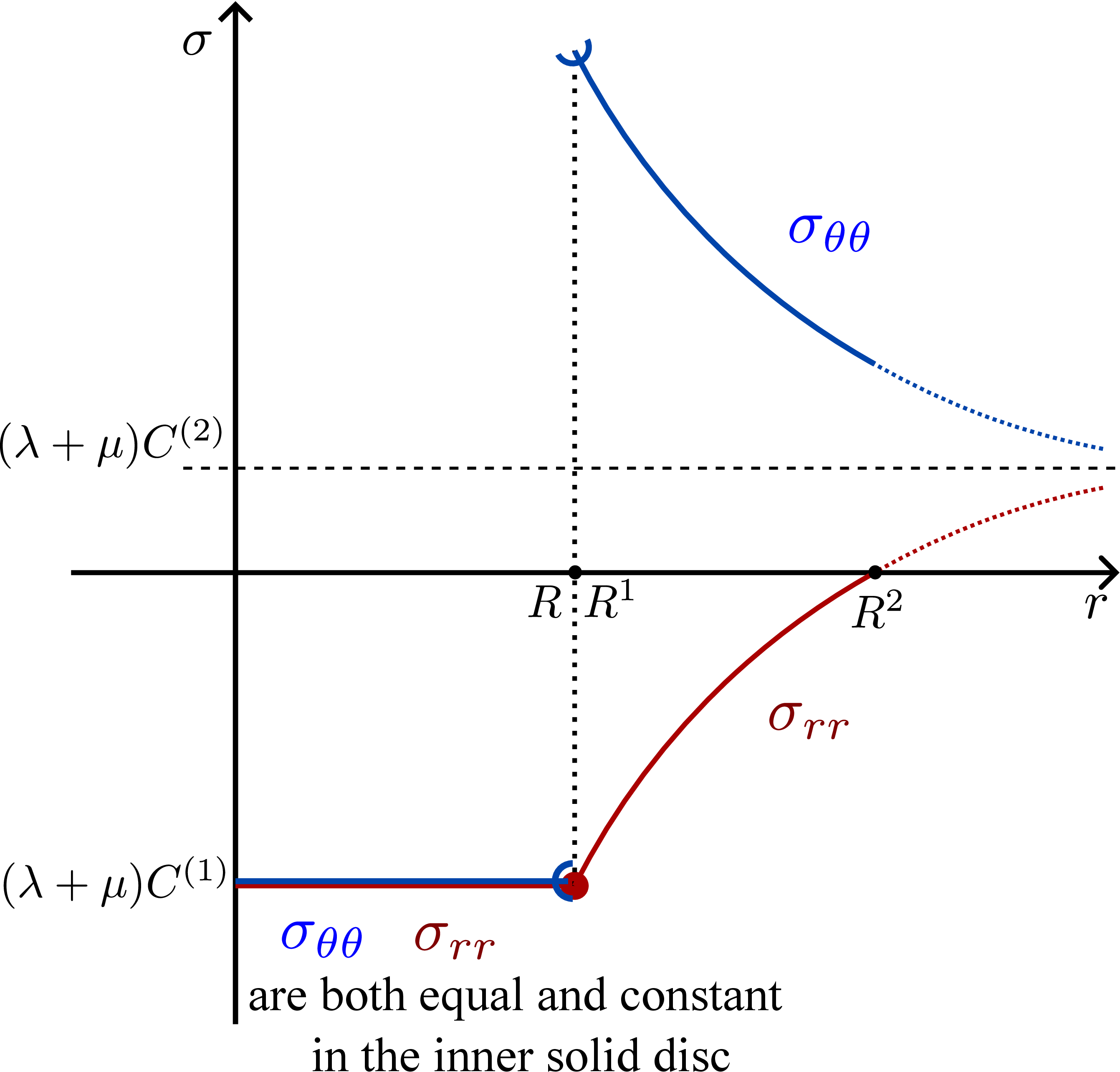
Solution:
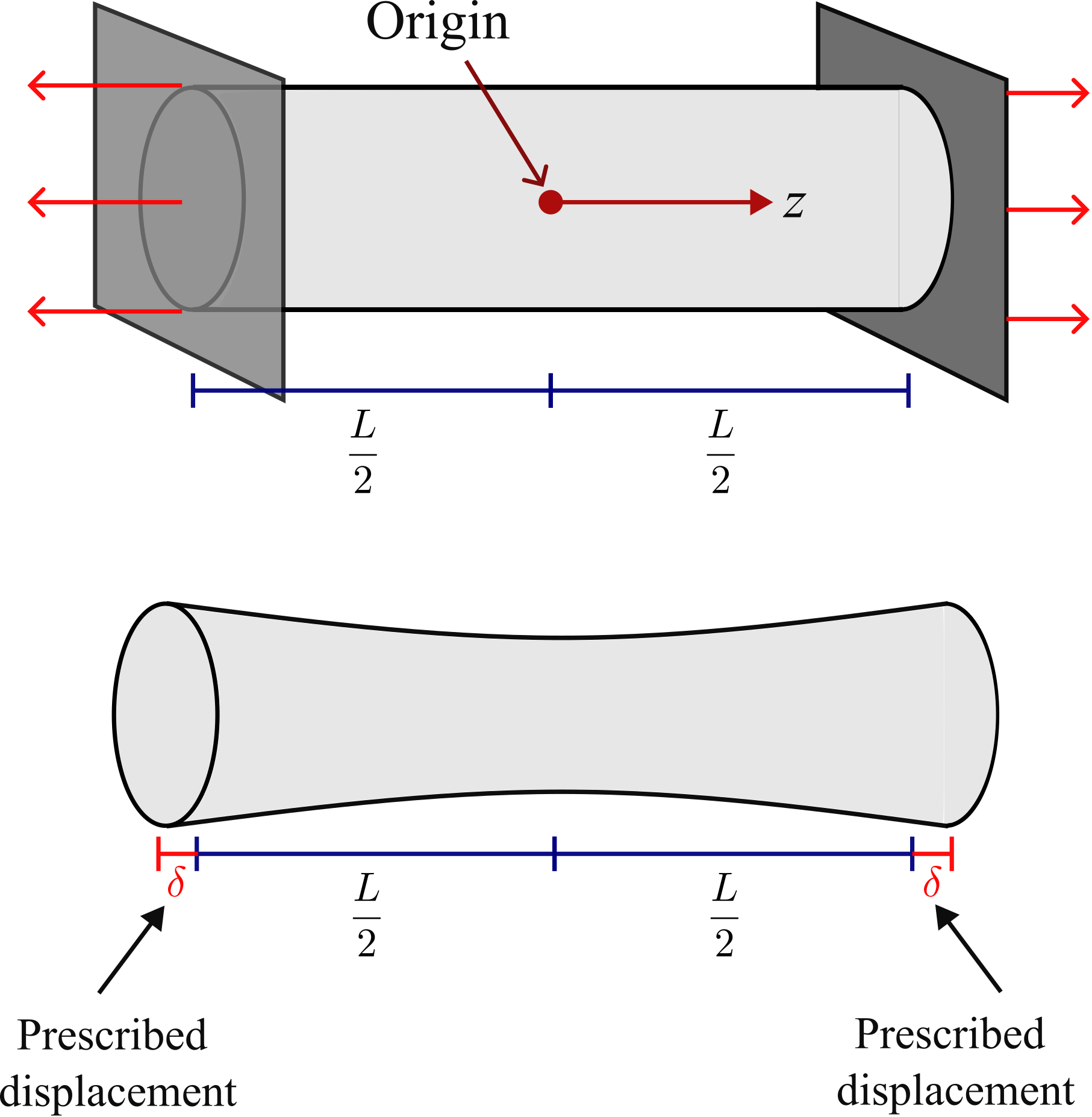
Notice that \(\gamma _{rz}\ne 0\) which is a departure from the case of uniform extension-torsion-inflation case. To obtain stress matrix, use \(\sigma _{ij}\;=\;\lambda \; tr\brc {\matr {\epsilon }}\delta _{ij}\;+\;2\mu \epsilon _{ij}\) which leads to \begin {align*} &\sigma _{rr}\;=\;\lambda \brc {\dfrac {\partial u_r}{\partial r}\;+\;\dfrac {u_r}{r}\;+\;\dfrac {\partial u_z}{\partial z}}\;+\;2\mu \dfrac {\partial u_r}{\partial r},\\ &\sigma _{\theta \theta }\;=\; \lambda \brc {\dfrac {\partial u_r}{\partial r}\;+\;\dfrac {u_r}{r}\;+\;\dfrac {\partial u_z}{\partial z}}\;+\;2\mu \dfrac {u_r}{r},\\ & \sigma _{zz}\;=\; \lambda \brc {\dfrac {\partial u_r}{\partial r}\;+\;\dfrac {u_r}{r}\;+\;\dfrac {\partial u_z}{\partial z}}\;+\;2\mu \dfrac {\partial u_z}{\partial z },\\ &\tau _{r \theta }\;=\;2G\epsilon _{r \theta }\;=\;0,\\ &\tau _{rz}\;=\;2G\epsilon _{r z}\;=\;G \dfrac {\partial u_r}{\partial z}\;,\;\tau _{\theta z}\;=\;0. \end {align*}
So, \(\theta \)-equation is automatically satisfied! It happened due to the assumption of axisymmetry which allows the reduction of equilibrium equation from the whole three-dimensional cylindrical domain to just its \(r-z\) plane.
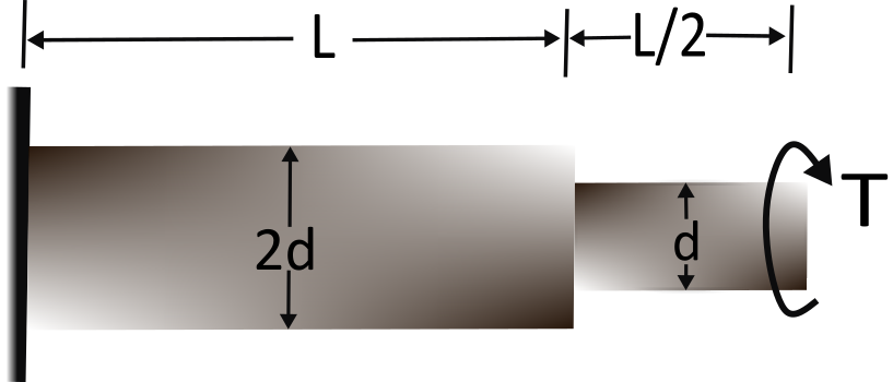
\(\underline {\nabla }\cdot ()=\frac {\partial }{\partial r}()\cdot \underline {e}_r+\frac {1}{r}\frac {\partial }{\partial \theta }()\cdot \underline {e}_{\theta }+\frac {\partial }{\partial z}()\cdot \underline {e}_z\).
Show that the divergence components so obtained have the same expression as the LHS of the components of stress equilibrium equation (without body force).
∗We remark that cylindrical coordinate system can otherwise be used also for general deformation of bodies having arbitrary shape.
†The formula for area \(A_z\) can be found either by actual integration of \(dA\) or by identifying the lengths in Figure 7.5b. The length of the curved centerline is \(r\Delta \theta \) (arc of radius \(r\) subtending an angle \(\Delta \theta \)) while the length of the straight edges is \(\Delta r\). As \(\Delta r\) and \(\Delta \theta \) are very small, the curved top face becomes a trapezoid when the cylindrical element becomes very small. The centerline of the curved face gives the average of the two sides of the trapezoid. Thus, the area of this face will be \(r\Delta r\Delta \theta \).
‡As the dimensions of the cylindrical element tends to 0, the curved edge becomes nearly a straight line.
§For a cuboid element, the areas of opposite faces are the same.
¶The superposition principle does not hold in nonlinear elasticity though which is the realm of large deformation problems.
ʺWe could have also applied pressure on the outer surface of the cylinder to analyze inflation, but here we will focus on pressure on the inner surface.
∗∗Our assumption that only \(u_{\theta }\) generates during torsion again holds good only when a small enough torque is applied to a beam. However, when torque applied is large, torsion can also generate radial contraction/expansion and axial elongation/contraction in beams. This happens solely due to nonlinearity and superposition principle does not hold then.
††As we started with axisymmetric displacement components, the strain components also become axisymmetric which further lead to axisymmetry of stress components. Due to this, the derivatives of stress components with respect to \(\theta \) vanish.
‡‡There are numerous examples of rotating cylinders in practice. Motors have constantly rotating shafts. Rotors in jet engines rotate continuously. Shafts in lathe machines also rotate constantly while under operating condition.
§§Note that pressure acts only on internal surface and hence it is not a body force
¶¶Keep in mind though that the radial coordinate \(r\) is physically realizable only between \(r_1\) and \(r_2\).
∗∗∗For cross-sections having irregular shape however, axisymmetry does not hold and we can then have non-zero \(\sigma _{rr}\) and \(\sigma _{\theta \theta }\) even during extension and torsion.
†††Note that a torque is usually shown by 2 parallel lines with an arrow head whereas a force vector is shown by a single line with an arrow head.