Having discussed the concepts of stress and strain, we will now talk about how they are related! We will
derive the most general form of linearly elastic stress-strain relationship and further discuss the special case
of isotropic materials. The chapter will conclude with a discussion on thermoelasticity.
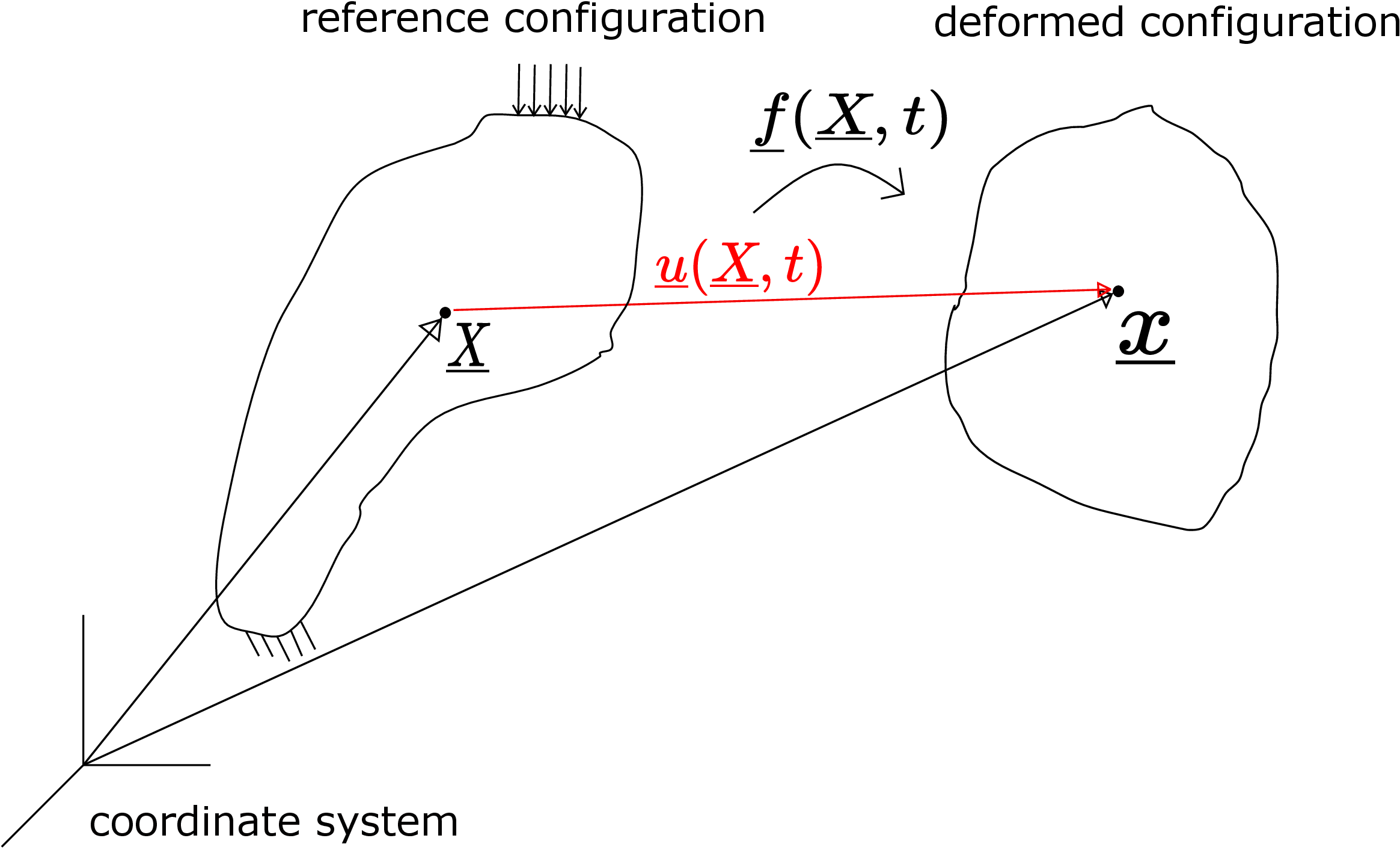
Let us first understand why do we need to relate stress with strain. Consider a body clamped at one part of
the boundary and acted upon by an external load on another part of its boundary as shown in Figure 6.1.
Any general point in the reference configuration (denoted by position vector \(\underline {X}\)) is displaced by \(\underline {u}(\underline {X},t)\) as shown in the figure. Usually, we are interested in knowing the final deformed shape of the body and the stress generated in it. The information of stress distribution within the body is important since it helps us to check if it is within the prescribed limits so that the body does not fail or fracture. In order to find stress in the body, we need to solve the following equations:
subject to problem specific boundary condition. We have nine unknown components of stress matrix in the three equation here. Using symmetry of stress matrix, the number of unknowns reduces to six. The body force components (\(b_1,b_2,b_3\)) are not unknowns as they are usually prescribed. For example, if gravitational body force is present, the body force will be \(\rho g\) pointing vertically downward. On the right hand side, we then have the components of acceleration which can be express in terms of displacement as we show now. The velocity of a particle located at \(\underline {X}\) in the reference configuration will be \begin {equation} \underline {v}(\underline {X},t)=\frac {\partial \underline {u}}{\partial t}\bigg |_{\underline {X}}. \end {equation} By keeping \(\underline {X}\) fixed here, We are ensuring that the particle does not change while taking the time derivative of displacement function. This is important otherwise the derivative obtained would not correspond to a specific particle. Let us denote the time derivatives with dots above the letter (\(n^{th}\) derivative has n dots), e.g.,
Thus, we can write velocity and acceleration of a particle at \(\underline {X}\) as follows:
This description of velocity and acceleration is also called Lagrangian description: whenever we describe velocity, acceleration or any other quantity of a particle in terms of the position of the particle in the reference configuration (X), we call it Lagrangian description.∗ We can now substitute the acceleration components in terms of time derivative of displacement in the equilibrium equation \eqref{6_equilibrium}, i.e.,
We can observe that it has six unknown stress components and three unknown displacement components. So, we have nine unknowns in total but there are only three equations. Thus, this system cannot be solved without the help of additional equations. We also know that we can express strain in terms of displacement as given below:
If we can somehow express stress in terms of strain, then indirectly, we have actually expressed stress in terms of displacement.† So, in equilibrium equations, everything will finally be in terms of the three unknown displacement components. This system of three equations in three variables can then be solved.
Our goal is to express stress in terms of strain, i.e., \(\underline {\underline {\sigma }}=\underline {\underline {\hat {\sigma }}}(\underline {\underline {\epsilon }})\). As stress and strain tensors are both symmetric, they have six independent components each. In general, each of the stress components depends on each of the strain components, i.e.,
The functional form of this dependence can be anything (e.g., linear, exponential, logarithmic etc.) and will vary from material to material. There is no physical law to derive this functional form and therefore mechanicians resort to experiments on real material specimen and data fitting technique to obtain these relations. As we can express any arbitrary function as a polynomial series using its Taylor’s series expansion, we can do the same for the above stress components about the zero strain state.‡ Let us explore it now. The Taylor’s expansion of \(\sigma _{ij}\) with respect to strain components will be as follows: \begin {equation} \sigma _{ij}(\epsilon _{kl})=\underbrace {\sigma _{ij}(\epsilon _{kl}=0)}_{\sigma _{ij}^0}+\sum _k\sum _l\frac {\partial \sigma _{ij}}{\partial \epsilon _{kl}}\epsilon _{kl}+\sum _k\sum _l\sum _m\sum _n \frac {1}{2!}\frac {\partial ^2 \sigma _{ij}}{\partial \epsilon _{kl}\partial \epsilon _{mn}}\epsilon _{kl}\epsilon _{mn}+... \end {equation} All the derivatives here have been evaluated at zero strain state, i.e., \(\epsilon _{kl}=0\). Also, all the indices run from 1 to 3. The first term (denoted as \(\sigma _{ij}^0\)) in the above expansion is the residual stress which is the stress in zero strain state or the reference configuration. As the reference configuration is typically chosen such that the stress in the body is zero in this state, we accordingly take \(\sigma _{ij}^0\) to be zero. The second term is linear in strain while the third term is quadratic in strain. We had earlier said that for this course, we will work with small strain components. Thus, we can neglect the terms which are quadratic or higher order in strain components as they will be much smaller than the linear term. Thus, we are left with \begin {equation} \label {6_linear_stress_strain_relation} \sigma _{ij}=\sum _{k=1}^3\sum _{l=1}^3\frac {\partial \sigma _{ij}}{\partial \epsilon _{kl}}\epsilon _{kl}. \end {equation} This is called linear stress-strain relation. We again remark that the derivatives in equation \eqref{6_linear_stress_strain_relation} are to be evaluated in the reference configuration. These derivatives have a special significance in solid mechanics: they denote the components of the stiffness tensor. It is a fourth order tensor because it has got four indices all running from 1 to 3 and is denoted by \(C_{ijkl}\): \begin {equation} C_{ijkl}=\frac {\partial \sigma _{ij}}{\partial \epsilon _{kl}}\bigg |_{\epsilon _{kl}=0}. \end {equation} Thus, we can write \begin {equation} \label {6_final_linear_relation} \boxed {\sigma _{ij}=\sum _k\sum _l C_{ijkl}~\epsilon _{kl}} \end {equation}
We can observe that \(C_{ijkl}\) has \(3^4=81\) terms since all the four indices go from 1 to 3. These 81 constants are material constants which vary from material to material. However, it turns out that these 81 constants are not all independent. Let us explore it now.
As \(\sigma _{ij}\) is symmetric, it implies that \begin {equation} \label {6_Minor_symmetry1} C_{ijkl}=C_{jikl}. \end {equation} For example, \(C_{1222}=C_{2122}\), \(C_{1323}=C_{3123}\). If this is not satisfied then if we work out the multiplication of the RHS in equation \eqref{6_final_linear_relation}, \(\sigma _{ij}\) will not come out to be equal to \(\sigma _{ji}\). Likewise, as \(\epsilon _{kl}\) is symmetric, one can choose \begin {equation} \label {6_Minor_symmetry2} C_{ijkl}=C_{ijlk}. \end {equation} This is because the multiplication in \eqref{6_final_linear_relation} only depends on \((C_{ijkl}+ C_{ijlk})/2\) part of \(C_{ijkl}\) due to symmetry of strain components as we show below:
In the last equality here, we have simply replaced \(\epsilon _{kl}\) in the last term with \(\epsilon _{lk}\) due to symmetry in strain components. However, this implies that the last two summations become exactly the same and hence cancel each other: just interchange the summation subscripts (\(k\to l,~l\to k\)) in the last summation. Equations \eqref{6_Minor_symmetry1} and \eqref{6_Minor_symmetry2} are together called minor symmetries of the stiffness tensor. By using equation \eqref{6_Minor_symmetry1}, out of the 9 combinations of \((i,j)\), only 6 are independent. Similarly, by using equation \eqref{6_Minor_symmetry2}, out of the 9 combinations of \((k,l)\), only 6 are independent. Thus, we have \(6\times 6=36\) independent components from the total 81 components. The number of independent constants reduces further upon using another kind of symmetry which is called Major symmetry.
This is another symmetry present in the stiffness tensor which comes from energy considerations. It implies \begin {equation} C_{ijkl}=C_{klij}. \end {equation} Let us prove it. First, let us look at the analogue of a spring.
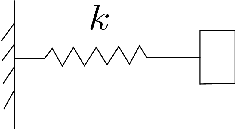
If the elongation of the spring is \(x\) and the spring constant is \(k\), the force \(F\) that gets generated in the spring is given by \begin {equation} F=kx \end {equation} while the energy stored in the spring is given by \begin {equation} \label {6_spring_energy} E=\frac {1}{2}kx^2=\frac {1}{2}(kx)x=\frac {1}{2}Fx. \end {equation} We also have \begin {equation} \label {6_spring_E_F_relation} \frac {\partial E}{\partial x}=kx=F. \end {equation} This is the case of a simple spring. We can think of a three-dimensional body as being made up of multiple springs. The strain components can be thought of as the elongation in an individual spring and the stress components can be thought of as the force that generates in that particular spring. The only difference here is that the force in a spring (\(\sigma _{ij}\)) not only depends on the strain in that spring but also on strains in other springs. For example, \(\sigma _{11}\) depends on \(\epsilon _{12},\epsilon _{13},\epsilon _{22},\epsilon _{23}\) and \(\epsilon _{33}\) too in addition to \(\epsilon _{11}\). Thus, a three-dimensional elastic body is just a more complicated/coupled set of springs. Using this analogy, we can also say that the energy is stored when a body deforms. This stored energy is called strain energy density (per unit volume). To get the total energy stored in a body, we can integrate the strain energy density over the entire volume of the body. Analogous to spring energy in \eqref{6_spring_energy}, we can write strain energy density \(E\) in a three-dimensional body as follows: \begin {equation} E(\text {strain energy/volume})=\frac {1}{2}\sum _i\sum _j\sigma _{ij}\epsilon _{ij}. \end {equation} As \(i\) and \(j\) go from 1 to 3, there are a total of 9 springs. Let us now substitute for \(\sigma _{ij}\) using linear stress-strain relation given in equation \eqref{6_final_linear_relation}:
This is the energy stored per unit volume in the body. Now, we can also obtain stress component \(\sigma _{mn}\) analogous to equation \eqref{6_spring_E_F_relation}, i.e.,
We have used the fact that \(C_{ijkl}\) is a constant and does not change with strain. Assuming that the strain components are independent of each other, the partial derivative of one component with respect to another will give 1 if they are the same and 0 otherwise. To express this mathematically, we need to use multiplication of two Kronecker Delta functions, e.g.,§
We thus have
As \(i\) and \(j\) are just used for summation and are dummy variables, we can change them to \(k\) and \(l\) respectively which yields
where
This \(\tilde {C}_{mnkl}\) has got major symmetry as shown below:
From this analysis, we can conclude that although equation \eqref{6_final_linear_relation} has a general \(C\) tensor, we can always work with an equivalent \(\tilde {C}\) which has both major and minor symmetries. Due to major symmetry, the number of independent constants in \(C_{ijkl}\) reduces further. We can think of a \(6\times 6\) matrix with the rows representing the values of \(C_{ijkl}\) corresponding to independent combinations of \((i,j)\) and the columns representing the values of \(C_{ijkl}\) corresponding to independent combinations of \((k,l)\), i.e., \begin {equation} \label {6_major_symmetry_matrix} \begin {bmatrix} C_{ijkl} \end {bmatrix}= \begin {bmatrix} C_{1111} & C_{1122} & C_{1133} & C_{1123} & C_{1113} & C_{1112}\\ C_{2211} & C_{2222} & C_{2233} & C_{2223} & C_{2213} & C_{2212}\\ C_{3311} & C_{3322} & C_{3333} & C_{3323} & C_{3313} & C_{3312}\\ C_{2311} & C_{2322} & C_{2333} & C_{2323} & C_{2313} & C_{2312}\\ C_{1311} & C_{1322} & C_{1333} & C_{1323} & C_{1313} & C_{1312}\\ C_{1211} & C_{1222} & C_{1233} & C_{1223} & C_{1213} & C_{1212} \end {bmatrix}. \end {equation} From major symmetry, we know that we can flip \((i,j)\) and \((k,l)\) which implies that the above matrix is symmetric. Thus, out of the 36 components here, only 21 are independent. We can summarize the reduction in number of independent components as follows: \begin {equation*} 81 (3^4)\xrightarrow {\text {Minor Symmetry}}36 (6^2)\xrightarrow {\text {Major Symmetry}}21. \end {equation*}
Although the stress tensor is written in a matrix form, one can also think of writing it as a \(6\times 1\) column formed by its six independent components. The sequence in which they are written is shown in Figure 6.3.
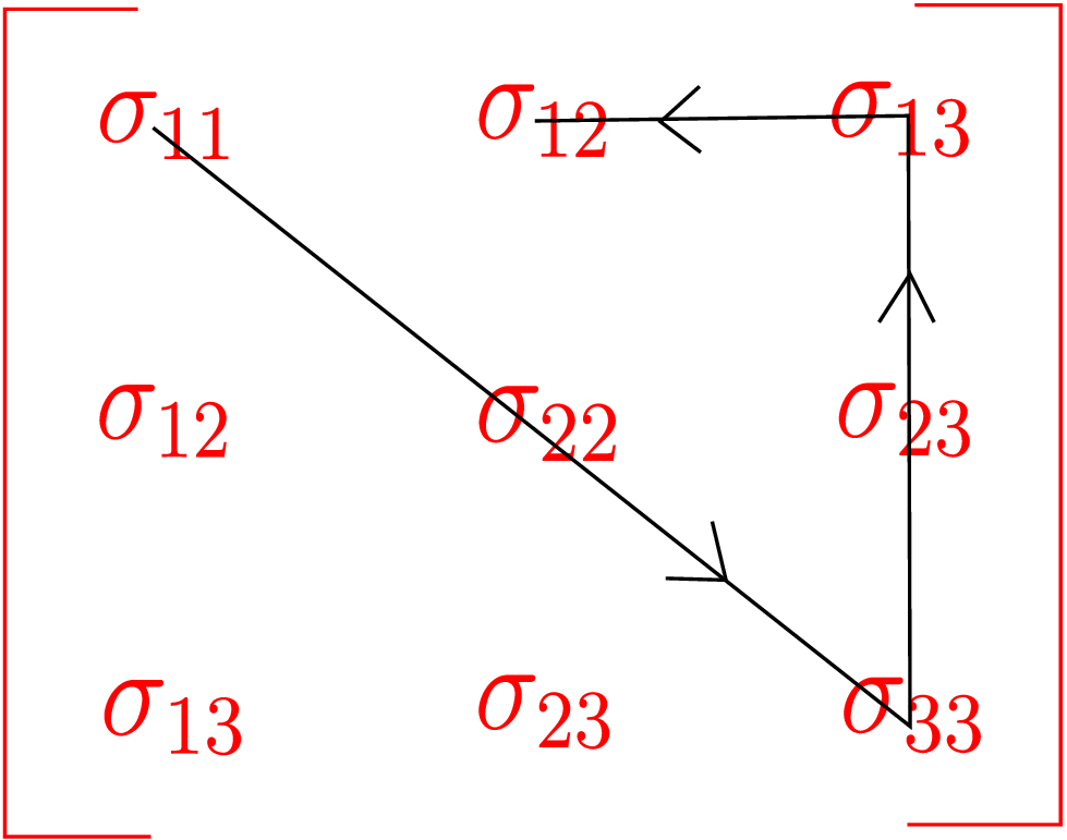
We first go along the diagonal starting from (1,1) component. Then we go up along the third column and then left along the first row. Thus, we obtain the following column form: \begin {equation} [\underline {\sigma }]= \begin {bmatrix} \sigma _{11}\\ \sigma _{22}\\ \sigma _{33}\\ \sigma _{23}\\ \sigma _{13}\\ \sigma _{12} \end {bmatrix}. \end {equation} This is also called the stress vector. We can follow the same steps to get the strain vector, i.e., \begin {equation} [\underline {\epsilon }] =\begin {bmatrix} \epsilon _{11}\\ \epsilon _{22}\\ \epsilon _{33}\\ 2\epsilon _{23}\\ 2\epsilon _{13}\\ 2\epsilon _{12} \end {bmatrix} =\begin {bmatrix} \epsilon _{11}\\ \epsilon _{22}\\ \epsilon _{33}\\ \gamma _{23}\\ \gamma _{13}\\ \gamma _{12} \end {bmatrix}. \end {equation} For linear stress-strain relation, there exists a matrix which relates the stress vector with the strain vector, i.e., \begin {equation} \begin {bmatrix} \sigma _{1}\\ \sigma _{2}\\ \sigma _{3}\\ \sigma _{4}\\ \sigma _{5}\\ \sigma _{6} \end {bmatrix}= \begin {bmatrix} \,\\ \quad \text {$6\times 6$ matrix}\quad \\ \,\\ \text {(formed by}\\ \text {$C_{ijkl}$)}\\ \,\\ \end {bmatrix} \begin {bmatrix} \epsilon _{1}\\ \epsilon _{2}\\ \epsilon _{3}\\ \epsilon _{4}\\ \epsilon _{5}\\ \epsilon _{6} \end {bmatrix}. \end {equation} This \(6\times 6\) matrix is called the stiffness matrix. It is the same matrix as in \eqref{6_major_symmetry_matrix} which is symmetric and contains 21 independent constants. We can also write the strain vector (\(\underline {\epsilon }\)) in terms of stress vector (\(\underline {\sigma }\)) using another \(6\times 6\) matrix: \begin {equation} \begin {bmatrix} \epsilon _{1}\\ \epsilon _{2}\\ \epsilon _{3}\\ \epsilon _{4}\\ \epsilon _{5}\\ \epsilon _{6} \end {bmatrix}= \begin {bmatrix} \,\\ \,\\ \quad \text {$6\times 6$ matrix}\quad \\ \,\\ \,\\ \,\\ \end {bmatrix} \begin {bmatrix} \sigma _{1}\\ \sigma _{2}\\ \sigma _{3}\\ \sigma _{4}\\ \sigma _{5}\\ \sigma _{6} \end {bmatrix}. \end {equation} This \(6\times 6\) matrix is called the compliance matrix which turns out to be the inverse of the stiffness matrix. Although, the most general material has 21 independent material constants, there are materials with additional symmetries. For example, isotropic materials have only two independent constants. We will discuss such materials next.
As the name suggests, isotropic materials have the same property in all directions. To understand what we mean, consider a body made up of isotropic material and stretch it at an arbitrary point along \(\underline {e}_1\) direction as shown in Figure 6.4.
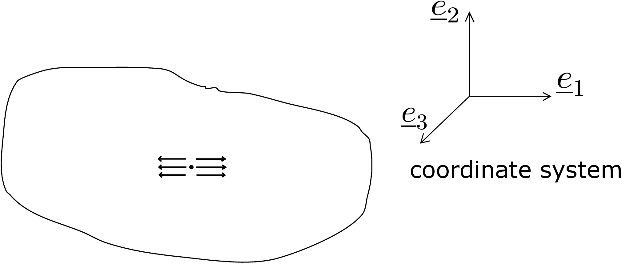
We have restricted the body in such a way that the deformation is not allowed in any direction other than \(\underline {e}_1\). Thus, the strain matrix at the point of interest has only \(\epsilon _{11}\) as the non-zero component, i.e., \begin {equation} \underline {\underline {\epsilon }}= \begin {bmatrix} \epsilon _{11} & 0 & 0\\ 0 & 0 & 0\\ 0 & 0 & 0 \end {bmatrix}. \end {equation} Using equation \eqref{6_final_linear_relation}, we can then write
We now do another experiment with the same body. However, this time instead of stretching along \(\underline {e}_1\), we stretch along \(\underline {e}_2\) as shown in Figure 6.5. We again constrain the body to not allow deformation in any direction except \(\underline {e}_2\).
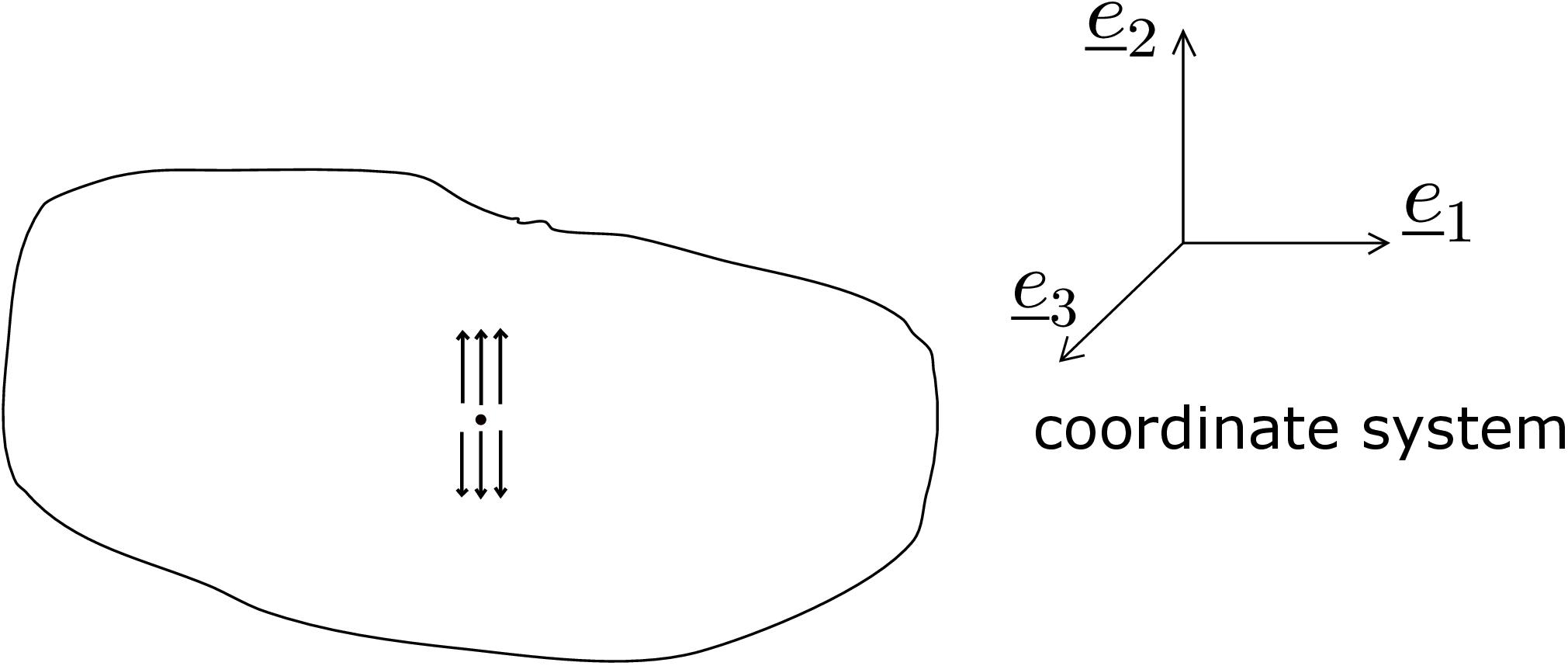
So, the new strain matrix at the point of interest will be \begin {equation} \underline {\underline {\epsilon }}= \begin {bmatrix} 0 & 0 & 0\\ 0 & \epsilon _{22} & 0\\ 0 & 0 & 0 \end {bmatrix}. \end {equation} We can thus write
As the material is isotropic, the response of the material, e.g., the stress generated in the two cases above should be the same if the strain applied is also the same. Thus, if \(\epsilon _{11}\) in the first case equals \(\epsilon _{22}\) in the second case, then \(\sigma _{11}\) in the first case should be the same as \(\sigma _{22}\) in the second case. On comparing equations \eqref{6_stress_11} and \eqref{6_stress_22}, we find that it is possible if and only if \(C_{1111}=C_{2222}\). Similarly, if we do the analysis for stretching along \(\underline {e}_3\), we can conclude that \begin {equation} C_{1111}=C_{2222}=C_{3333}. \end {equation} These are additional constraints on the coefficients of the stiffness tensor for isotropic materials. They are not covered by either minor or major symmetries. In fact, a rigorous analysis proves that there are several other constraints in this case all of which finally lead to only two independent constants for the stiffness tensor of isotropic materials. This also means that for isotropic materials, we just have to do two independent experiments to fully characterize its material response (for a general material, we will need to do 21 experiments!). When we work out the stress-strain relation for isotropic materials using a rigorous mathematical derivation, we get
Here (\(\lambda ,\mu \)) are called the Lame’s constants. Let us consider the case when \(i=j=1\), i.e., \begin {equation} \sigma _{11}=\lambda (\epsilon _{11}+\epsilon _{22}+\epsilon _{33})+2\mu \epsilon _{11}. \end {equation} Comparing with equation \eqref{6_final_linear_relation}, we can see that \(C_{1111}\) (the constant relating \(\sigma _{11}\) and \(\epsilon _{11}\)) will be given by the coefficient of \(\epsilon _{11}\), i.e., \begin {equation} \label {6_isotropic_C_1111} C_{1111}=\lambda +2\mu . \end {equation} Likewise, we can also deduce \begin {equation} C_{1122}=C_{1133}=\lambda . \end {equation} Similarly, using equation \eqref{6_isotropic_stress_in_terms_of_strain}, we can write \begin {equation} \sigma _{22}=\lambda (\epsilon _{11}+\epsilon _{22}+\epsilon _{33})+2\mu \epsilon _{22}\Rightarrow C_{2222}=\lambda +2\mu . \end {equation} Comparing this with equation \eqref{6_isotropic_C_1111}, we can verify that \(C_{1111}=C_{2222}\). When \(i\neq j\), the first term in equation \eqref{6_isotropic_stress_in_terms_of_strain} becomes zero due to the Kronecker delta function present there. For example, \begin {equation} \label {6_isotropic_sigma_12} \sigma _{12}=2\mu \epsilon _{12}=\mu (\epsilon _{12}+\epsilon _{21})\Rightarrow C_{1212}=C_{1221} = \mu . \end {equation} Equation \eqref{6_isotropic_stress_in_terms_of_strain} gives stress in terms of strain. Alternatively, we can use another form where strain is expressed in terms of stress. It is also called the isotropic three-dimensional Hooke’s law of elasticity¶ as shown below:
In this representation, we have three constants: \(E\) denoting Young’s modulus of elasticity, \(\nu \) denoting Poisson’s Ratio and \(G\) denoting shear modulus of elasticity. As we know that isotropic materials have only two independent constants, there is a relation between \(E\), \(G\) and \(\nu \) given by \begin {equation} \label {6_strain_form_final_equation} G=\frac {E}{2(1+\nu )}. \end {equation} Finally, comparing equation \eqref{6_strain_form_gamma_12} with equation \eqref{6_isotropic_sigma_12}, we can also note that \begin {equation} \mu =G. \end {equation}
Let us consider equations \eqref{6_strain_form_epsilon_11}, \eqref{6_strain_form_epsilon_22} and \eqref{6_strain_form_epsilon_33}. We can see that the normal strain in one direction not only depends on the normal stress component in that direction but also on normal stress components in other two directions. To understand its physical relevance, we can think of a simple experiment. Suppose that we have a rectangular beam of length \(L\), breadth \(B\) and height \(H\) as shown in Figure 6.6.
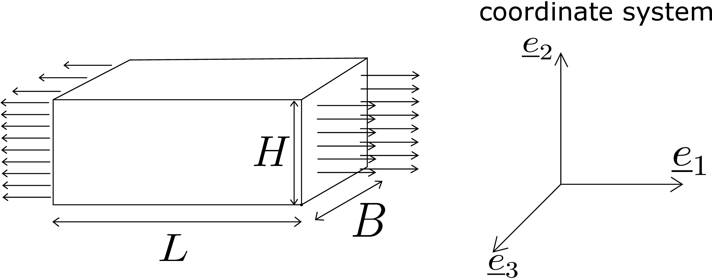
The beam is oriented such that its length is along \(\underline {e}_1\), its height along \(\underline {e}_2\) and its breadth along \(\underline {e}_3\). We apply force on the left and right faces to stretch the beam. So, \(\sigma _{11}\) will be non-zero while the shear components \(\sigma _{12}\) and \(\sigma _{13}\) will be zero (force applied is in just \(\underline {e}_1\) direction). Also, as we are not applying any force on the lateral surfaces (\(\underline {e}_2\) and \(\underline {e}_3\) planes), there is no stress on them. In fact, any internal section with normal along \(\underline {e}_2\) and \(\underline {e}_3\) will not have any traction component. The state of stress in this case will then be \begin {equation} \begin {bmatrix} \sigma _{11} & 0 & 0\\ 0 & 0 & 0\\ 0 & 0 & 0 \end {bmatrix}. \end {equation} This stress will lead to some strain in the body. We know that \(\epsilon _{11}\) is generated because the length of the beam changes. However, \(\epsilon _{22}\) and \(\epsilon _{33}\) also generate: due to stretching in one direction, there will be contraction in the other two directions. We can physically realize this when we stretch a rubber bar or a soft bar along its axis - their cross-section dimension reduces. But, there will be no shear strain generated if we are careful in stretching uniformly. Thus, the state of strain in the rectangular beam of Figure 6.6 will be \begin {equation} \begin {bmatrix} \epsilon _{11} & 0 & 0\\ 0 & \epsilon _{22} & 0\\ 0 & 0 & \epsilon _{33} \end {bmatrix}. \end {equation}
We know that longitudinal strain \(\epsilon _{jj}\) is given by \(\dfrac {\partial u_j}{\partial X_j}\). Assuming uniform strain field in the bar, the local strain will be equal to the global strain. Thus, we have
If we now draw the graph of \(\sigma _{11}\) vs \(\epsilon _{11}\) for the above experiment by measuring the change in length, we will get a curve as shown in Figure 6.7.
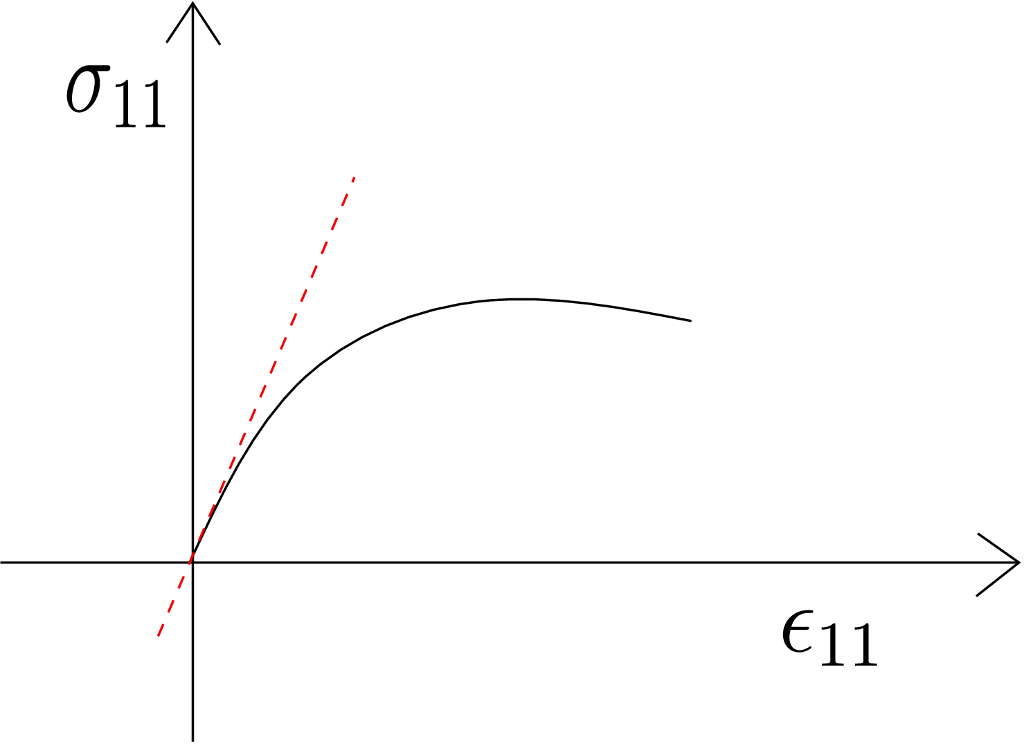
The initial slope of this graph (shown as the red dotted line) gives us the Young’s Modulus \(E\), i.e., \begin {equation} E=\frac {\partial \sigma _{11}}{\partial \epsilon _{11}}\bigg |_{\epsilon _{11}=0}. \end {equation} While computing this derivative, we should not have \(\sigma _{22}\) or \(\sigma _{33}\) present. Essentially, the bar should be stretched in such a way that it can freely shrink in lateral directions. We can also prove the above formula using equation \eqref{6_strain_form_epsilon_11}. Upon putting the condition of the experiment into it, i.e., \(\sigma _{22}=\sigma _{33}=0\), we will get \begin {equation} \sigma _{11}=E\epsilon _{11}. \end {equation} From this equation, we can see that the slope of the graph of \(\sigma _{11}\) vs \(\epsilon _{11}\) will give us \(E\). A point to note here is that equation \eqref{6_strain_form_epsilon_11} gives us the slope of \(\sigma _{11}\) vs \(\epsilon _{11}\) plot to be a constant. But in reality, the slope is not a constant as evident from Figure 6.7. This is because the linear stress strain relation \eqref{6_strain_form_epsilon_11} works only for small strains. On the other hand, Figure 6.7 shows the curve even for large strains and this is the reason that we had to take the slope of this graph at \(\epsilon _{11}=0\).
The Poisson’s ratio of a material is also obtained from uniaxial tension test and is defined as \begin {equation} \label {6_Poisson_basic} \nu =-\frac {\text {induced lateral normal strain}}{\text {imposed longitudinal strain}}. \end {equation} In the rectangular bar experiment shown in Figure 6.6, we are directly imposing longitudinal strain in \(\underline {e}_1\) direction and this, in turn, induces strains along \(\underline {e}_2\) and \(\underline {e}_3\) directions. For an isotropic body, the lateral strains in these two directions will be equal. Thus, the Poisson’s ratio for this experiment will be \begin {equation} \label {Poisson_experiment} \nu =-\frac {\epsilon _{22}}{\epsilon _{11}}=-\frac {\epsilon _{33}}{\epsilon _{11}}. \end {equation} We can also derive this from stress-strain relation. Consider equations \eqref{6_strain_form_epsilon_11} and \eqref{6_strain_form_epsilon_22}. Let us substitute the condition of experiment, i.e., \(\sigma _{22}=\sigma _{33}=0\). From equation \eqref{6_strain_form_epsilon_11}, we get \begin {equation} \label {6_Poisson_1} \epsilon _{11}=\frac {1}{E}\sigma _{11} \end {equation} while from equation \eqref{6_strain_form_epsilon_22}, we get
We thus get the same formula for the Poisson’s ratio as in \eqref{Poisson_experiment}.
From equation \eqref{6_strain_form_gamma_12}, we can see that shear modulus is given by \begin {equation} G=\frac {\tau _{12}}{\gamma _{12}}. \end {equation} So, if we can induce shear in a body and measure the corresponding shear stress, the ratio of stress to strain will give us the shear modulus. Motivated by this, let us conduct another experiment with the rectangular bar. The bar is fixed at the bottom face and we apply shear force along \(\underline {e}_1\) on the top face (face with normal along \(\underline {e}_2\)) as shown in Figure 6.8.
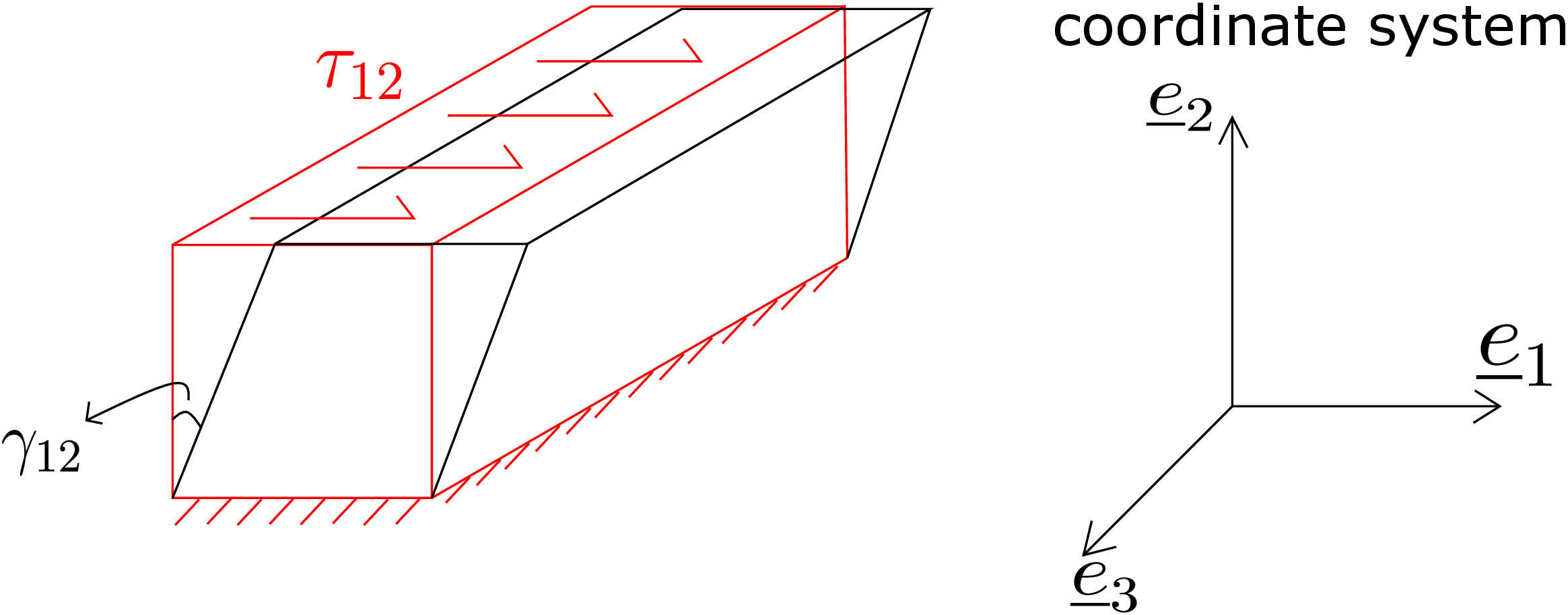
This effectively induces shear stress \(\tau _{12}\) in the body. Due to this, the bar shears: the initially perpendicular edges of the front face get inclined generating shear strain \(\gamma _{12}\) (as shown in Figure 6.8). If we draw the plot for \(\tau _{12}\) vs \(\gamma _{12}\), we get a representative curve as shown in Figure 6.9.
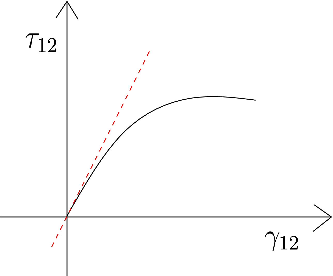
The initial slope of this curve gives us shear modulus, i.e., \begin {equation} G=\frac {\tau _{12}}{\gamma _{12}}\bigg |_{\gamma _{12}\to 0}. \end {equation} Again, the initial slope is measured because linear relations are valid only for small shear strains.
We have discussed Young’s modulus of elasticity and shear modulus of elasticity. The Young’s modulus relates normal strain with normal stress while shear modulus relates shear strain with shear stress. We will now discuss about bulk modulus of elasticity which relates volumetric strain with volumetric stress/ equivalent pressure. When we apply pressure to a fluid (liquid/gas), its volume decreases. This decrease can be quantified by volumetric strain given by \begin {equation} \text {Volumetric Strain}=\frac {\Delta V}{V}. \end {equation} If a pressure change of \(\Delta P\) generates volumetric strain \(\dfrac {\Delta V}{V}\) in a fluid, the bulk modulus is then given by \begin {equation} \label {6_bulk_liquid} K_{fluid}=-\frac {\Delta P}{\Delta V/V}. \end {equation} For solids, \(\dfrac {\Delta V}{V}\) is nothing but the volumetric strain discussed earlier, i.e., \begin {equation} \frac {\Delta V}{V}=tr\Big (\underline {\underline {\epsilon }}\Big )=\epsilon _{11}+\epsilon _{22}+\epsilon _{33}. \end {equation} The equivalent of pressure in solids, as discussed in a preceding chapter, is obtained from the hydrostatic part of stress tensor and is given by \begin {equation} p_{eq}=-\frac {I_1}{3}. \end {equation} So, along the lines of \eqref{6_bulk_liquid}, we can finally write \begin {equation} \label {6_K_initial} K_{solids}=-\frac {-I_1/3}{tr\Big (\underline {\underline {\epsilon }}\Big )}=\frac {1}{3}\,\frac {tr\Big (\underline {\underline {\sigma }}\Big )}{tr\Big (\underline {\underline {\epsilon }}\Big )}. \end {equation} Let us use the three-dimensional Hooke’s law to obtain a formula for the above quantity. Adding equations \eqref{6_strain_form_epsilon_11}, \eqref{6_strain_form_epsilon_22} and \eqref{6_strain_form_epsilon_33}, we get
This is a very important relation. Firstly, it tells us that the bulk modulus is not an independent constant. If we know Young’s modulus and Poisson’s ratio, we can also obtain bulk modulus using above relation. Secondly, this relation also gives an upper limit for the Poisson’s ratio as discussed below.
The Poisson’s ratio is usually positive. There is a recent surge in interest though in developing materials having
negative Poisson’s ratio which are called auxetic materials. We can deduce from equation \eqref{6_K_final} that
when \(\nu \) is very close to \(\frac {1}{2}\), the bulk modulus becomes very large. For such materials, if we apply a large amount
of equivalent pressure, the volumetric strain induced in the body would still be very small (also see
\eqref{6_bulk_liquid}). This signifies incompressibility. Thus, \(\nu \to \frac {1}{2}\) corresponds to the incompressible limit. If this limit
is crossed, \(K\) will become negative which is not physically meaningful.
To obtain the lower limit for the Poisson’s ratio, we can use equation \eqref{6_strain_form_final_equation}, i.e., \begin {equation} \label {6_shear_modulus} G=\frac {E}{2(1+\nu )}. \end {equation}
From the rectangular beam experiment in Figure 6.6 and Figure 6.8, we can observe that when we apply a
positive \(\sigma _{11}\), \(\epsilon _{11}\) should be positive and when we apply a positive \(\tau _{12}\), \(\gamma _{12}\) should be positive. So, Young’s modulus
and shear modulus are both positive quantities. As both the LHS and the numerator of the RHS in
equation \eqref{6_shear_modulus} are positive, the denominator of the RHS must also be positive, i.e.,
We thus have the following theoretical limit for the Poisson’s ratio: \begin {equation} \boxed {-1<\nu \leq \frac {1}{2}} \end {equation}
Let us think of modeling stress-strain relationship when the temperature of a material is also changing. When we heat a body, it simply expands with no stress developing in it. This expansion leads to an extra strain called thermal strain (\(\epsilon _T\)) which does not induce any stress in the body. It turns out that
Here \(\Delta T\) denotes the temperature change and the proportionality constant \(\alpha \) is called the thermal expansion coefficient. As this strain does not generate any stress in the body, it is subtracted from total strain to get the part of strain (also called elastic strain) which generates stress. This implies
The temperature change only affects normal strains and has no effect on shear strains. This is because only the length of line elements change with temperature and not the angle between line elements. Thus, the shear stress-shear strain relations remain unaffected, i.e.,
The equations \eqref{11_normal_thermoelastic} and \eqref{11_shear_thermoelastic} together constitute the isotropic three-dimensional thermoelastic stress-strain relation.
There are materials which are not isotropic but commonly seen in nature. For example, consider the material shown in Figure 6.10a: a family of parallel fibers are included in otherwise isotropic materials to make them fiber reinforced. As a result of this, the Young’s modulus of the final material in the direction of the fiber becomes different to the Young’s modulus in the direction perpendicular to fibers. Actually, in all directions transverse to fibers, it has the same young’s modulus but different from the one along the fiber. Due to this directional dependence, the material no longer remains isotropic. Such materials are called transversely isotropic materials and they require 5 independent material constants to fully characterize their material response. Let us now put another family of fibers in the material but perpendicular to the initial family as shown in Figure 6.10b.
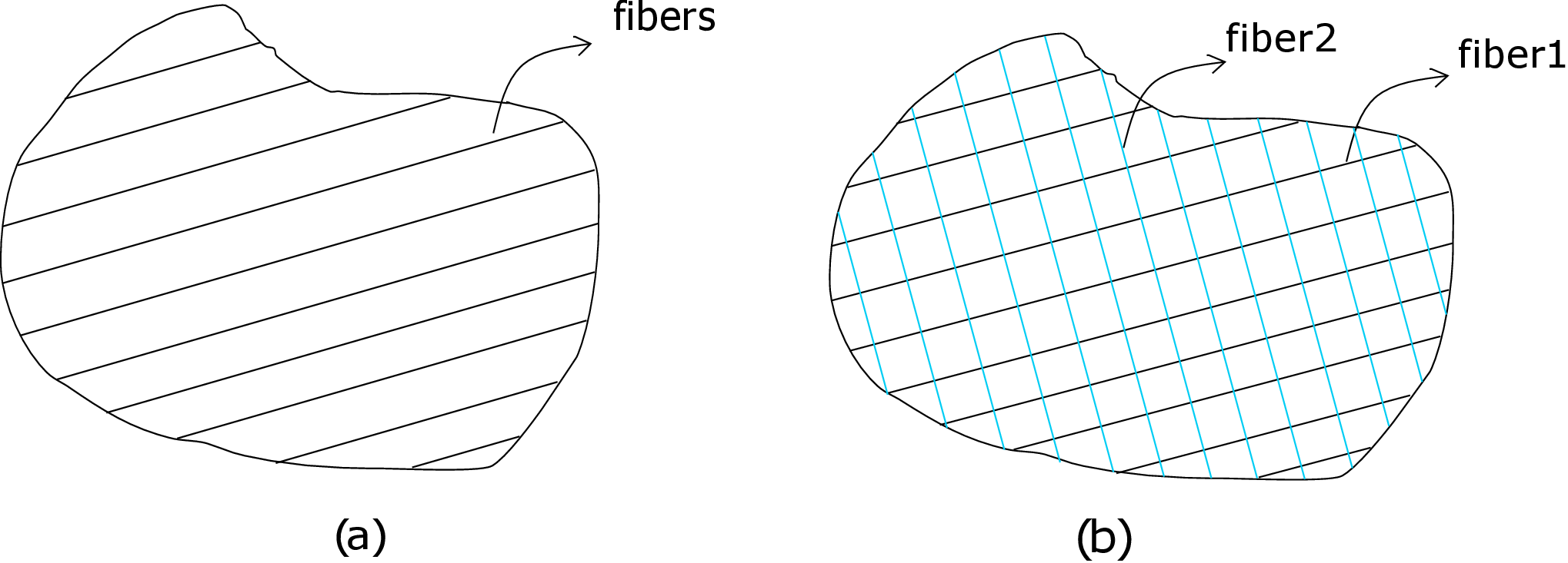
Assume the two fibers have different properties. So, the Young’s modulus along the two fibers will be different. In fact, the Young’s modulus in the direction perpendicular to both the fibers will also be different. Such materials are called orthotropic materials and they have 9 independent constants. Wood is an example of orthotropic materials.
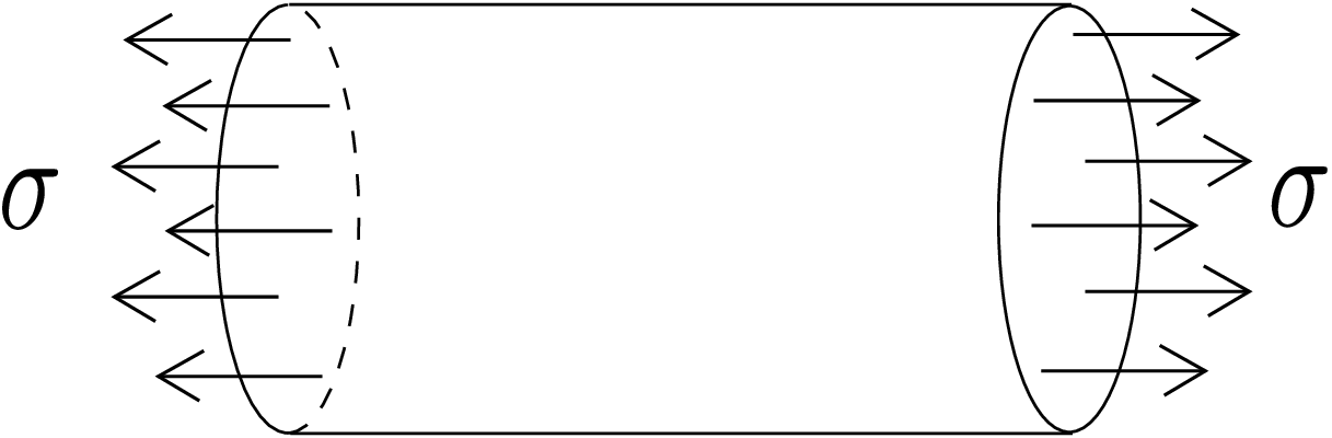
The discussion as of now were confined to elastic materials in which stress depends only on strain. Furthermore, if we somehow remove stress from the body, the body gets back to the original stress-free configuration. There are other materials however in which stress not only depends on strain but also on strain rate. Such materials are called viscoelastic. Then, there are viscous fluids in which stress depends only on strain rate and not on strain. There are also materials in which strain does not vanish upon removing the applied load. Essentially, such materials do not come back to their original shape upon removal of the applied load. For example, consider a steel bar on which a uniformly distributed load \(\sigma \) is applied at both its ends as shown in Figure 6.11.
We have shown the applied stress \(\sigma \) vs. the longitudinal strain \(\epsilon \) curve in Figure 6.12a.
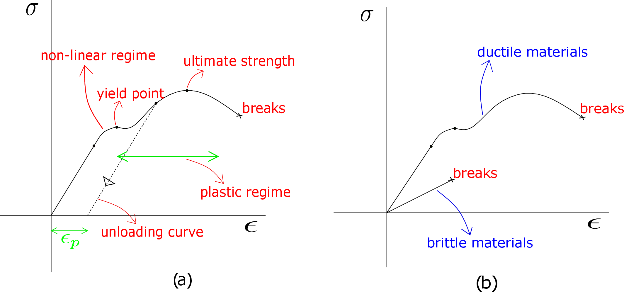
Initially, this curve is a straight line. This is the regime where linear stress-strain relationship holds. However, the curve does not remain linear throughout. The curved part up to the inflexion point, is the regime of non-linear stress-strain relation because the slope of the curve is changing in this regime. The body is still elastic in this regime which implies if the applied load is removed, the same curve is traced in the backward direction. As we keep increasing the load, there comes a point where the body yields, i.e., the beam elongates a lot even with very small increment in the applied load. The beam eventually breaks. The regime between the yield point and the breaking point is called the plastic regime. If we decrease the applied load in this regime, the original curve is not traced back as shown in the figure. Hence, when the stress becomes zero, the body retains some strain. This strain is called plastic strain (\(\epsilon _p\)). The yielding behavior is common in metals which give them ductile property. On the other hand, we also have brittle materials like glass which does not exhibit any yielding. They have a different stress-strain relationship (see Figure 6.12b).
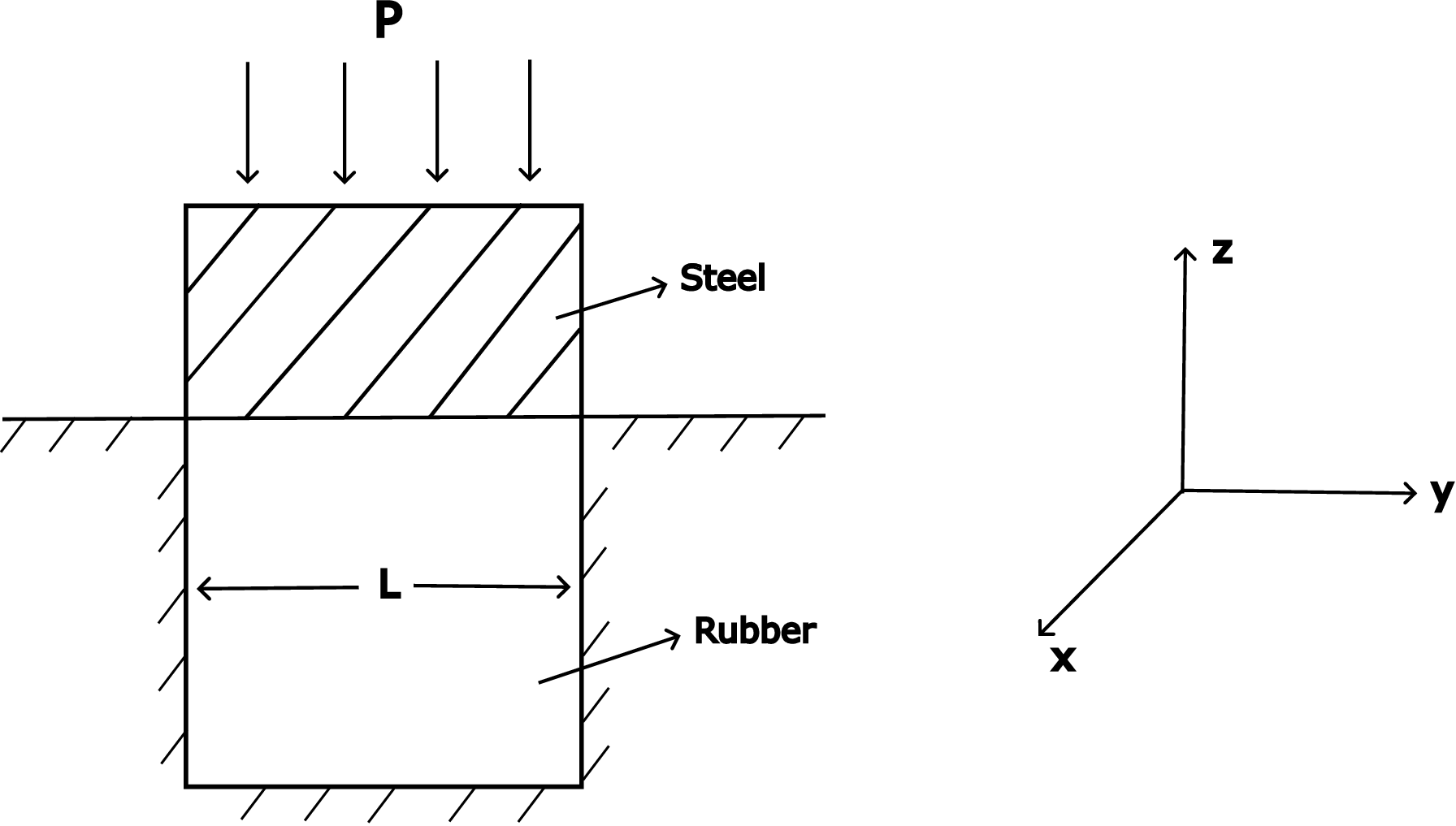
Solution: Let us neglect the weight of the rubber block in comparison to the steel block. Observe that the rubber
block is constrained against expanding in \(x\) and \(y\)-directions and can only displace vertically along \(z-\)direction. This
implies that
\[u_x=0,\; u_y=0, \; u_z(x,y,z).\]
Furthermore since the applied pressure is uniform, the vertical displacement \(u_z\) can be assumed to be independent of \(x\)
and \(y\) coordinates, i.e.,
\[u_z(x,y,z)\;=u_z(z).\]
Accordingly, the strain matrix becomes
\[\sbk {\matr {\epsilon }}\;=\; \begin {bmatrix} 0 & 0 & 0\\ 0 & 0 & 0\\ 0 & 0& \epsilon _{zz} \end {bmatrix}.\]
Next we want to obtain the stress components. Treating rubber as an isotropic linear elastic material, one
obtains:
\[ \tau _{xy}\;=\;\dfrac {\gamma _{xy}}{G}\;=\;0, \;\; \tau _{xz}\;=\;\dfrac {\gamma _{xz}}{G}\;=\;0, \;\; \tau _{yz}\;=\;\dfrac {\gamma _{yz}}{G}\;=\;0.\]
As of now, the remaining unknowns are \(\sigma _{xx},\;\sigma _{yy},\; \sigma _{zz}, \) and \(\epsilon _{zz}\). From the symmetry of the problem, we can say that \(\sigma _{xx}=\sigma _{yy}\)
as the same reaction is generated from steel walls in both directions. Note that even though \(\epsilon _{xx} = 0\) and \(\epsilon _{yy} = 0\),
it does not translate to \(\sigma _{xx}\) and \(\sigma _{yy}\) being zero. Physically, as the steel cavity constrains the rubber cube
from expanding, in the process, the wall of the steel cavity applies a constraining traction on the \(x-\)
and \(y-\) faces of the rubber cube leading to non-zero \(\sigma _{xx}\) and \(\sigma _{yy}\). Using stress-strain relations, one can further
write:
\[\cancelto {0}{\epsilon _{xx}}\;=\;\dfrac {1}{E}\sbk {\sigma _{xx}\;-\;\nu \brc {\cancelto {\sigma _{xx}}{\sigma _{yy}}\;+\;\sigma _{zz}}} \Rightarrow ~\sigma _{xx} \;(=\sigma _{yy})\;=\;\dfrac {\nu \sigma _{zz}}{\brc {1\;-\;\nu }}.\]
Let’s now use traction boundary condition for finding \(\sigma _{zz}\). Denoting the mass density of steel block as \(\rho \) and its height as
\(h\), the total traction applied on the top face of the rubber block can be equated to internal traction in the rubber
block there, i.e.,
\begin {align*} \matr {\sigma } ~\ve {e}_3 \;=\;\brc {\rho gh \;+\;p}\brc {-\ve {e}_3}~ \text {or}~\begin {bmatrix} \tau _{xz}\\ \tau _{yz}\\ \sigma _{zz} \end {bmatrix} \;&=\;\begin {bmatrix} 0 \\ 0 \\ -\brc {\rho gh\;+\;p} \end {bmatrix} \Rightarrow \;\sigma _{zz}\;=\;-\brc { p\;+\;\rho gh}. \end {align*}
Note that \(\sigma _{zz}\) calculated above is valid just at the top boundary surface of rubber cube. However, for this case, \(\sigma _{zz}\) is the same throughout the body (if we ignore the weight of the rubber block). This can be proved using equilibrium equations as shown below: \begin {align*} \frac {\partial \sigma _{zz}}{\partial z} + \frac {\partial \cancelto {0}{\tau _{zx}}}{\partial x} + \frac {\partial \cancelto {0}{\sigma _{zy}}}{\partial y} + \cancelto {0}{b_z} = \cancelto {0}{\rho a_z} \Rightarrow \frac {\partial \sigma _{zz}}{\partial z} =0 ~ \text {or}~\sigma _{zz} = \text {constant}. \end {align*}
Hence \(\sigma _{zz} = -\brc {p\;+\;\rho gh}\) is valid throughout the rubber cube. Therefore \(\sigma _{xx}\;=\;\sigma _{yy}\; = -\dfrac {\nu \brc {p\;+\rho gh}}{\brc {1\;-\;\nu }}.\) Moreover \begin {align*} \begin {split} \epsilon _{zz}\;&=\;\dfrac {1}{E}\sbk {\sigma _{zz}\;-\;\nu \brc {\sigma _{xx}\;+\;\sigma _{yy} }}=\; \dfrac {1}{E}\sbk {\sigma _{zz}\;-\;2\nu \sigma _{xx}}\\ &=\; \dfrac {1}{E}\sbk {\sigma _{zz}\;-\;\dfrac {2\nu ^2}{\brc {1\;-\;\nu }} \sigma _{zz}}=\; \dfrac {1}{E}\brc {\dfrac {1-\nu - 2\nu ^2}{1\;-\;\nu }}\sigma _{zz}. \end {split} \end {align*}
(b) Volumetric strain: \begin {align*} \begin {split} \epsilon _{v}\;=\;\epsilon _{xx}\;+\;\epsilon _{yy}\;+\;\epsilon _{zz} =\;0\;+\;0\;+\;\epsilon _{zz} =-\dfrac {1}{E}\brc {\dfrac {1-\nu -2\nu ^2}{1\;-\;\nu }}\brc {p\;+\;\rho gh}. \end {split} \end {align*}
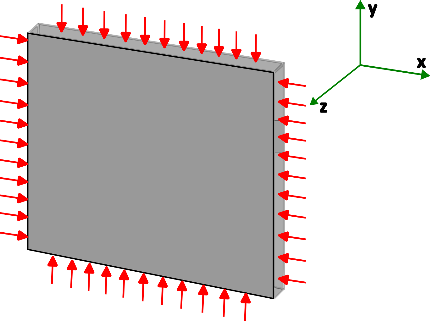
Assuming the material to be isotropic, find out the remaining components of strain matrix. Also obtain change in area divided by original area of the face of the plate (\(z\)-plane).
Solution: To determine \(\epsilon _{xx}\), \(\epsilon _{yy}\), \(\gamma _{xy}\), \(\gamma _{yz}\) and \(\gamma _{zx}\), we first use stress-strain relation for isotropic materials: \[\gamma _{xy}\;=\;\dfrac {\tau _{xy}}{G}\;=\;0\] and similarly \[ \gamma _{yz}\;=\;\gamma _{zx}\;=\;0.\] Using the following relation, we then get a relation between \(\sigma _{xx}\) and \(\sigma _{zz}\): \begin {align*} \cancelto {0}{\epsilon _{zz}}\;&=\;\dfrac {1}{E}\sbk {\sigma _{zz}\;-\;\nu \brc {\sigma _{xx}\;+\;\sigma _{yy}}} \\ \Rightarrow \;\;\sigma _{zz}\;&=\;\nu \brc {\sigma _{xx}\;+\;\sigma _{yy}} ~\text {or}~ \sigma _{zz}\;=-2\nu p. \end {align*}
Note that \(\sigma _{zz}\) turns out to be negative meaning it is under compression in thickness direction. To obtain \(\epsilon _{xx}\) and \(\epsilon _{yy}\), we use rest of the stress-strain relation: \begin {align*} \epsilon _{xx}\; =\;\dfrac {1}{E}\sbk {\sigma _{xx}\;-\;\nu \brc {\sigma _{zz}\;+\;\sigma _{yy}}}, ~ \epsilon _{yy}\;=\;\dfrac {1}{E}\sbk {\sigma _{yy}\;-\;\nu \brc {\sigma _{xx}\;+\;\sigma _{zz}}} \end {align*}
which leads to \begin {align*} \begin {split} \epsilon _{xx}\;=\;\dfrac {1}{E}\sbk {-p\;-\;\nu \brc {-2\nu p\;-\;p}} =\;\dfrac {-p}{E}\sbk {1\;-\;\nu \brc {2\nu \;+\;1}} =\;\dfrac {-\brc {1\;-\;\nu \brc {2\nu \;+\;1}}}{E}p. \end {split} \end {align*}
Also, we get \(\epsilon _{yy}\;=\;\epsilon _{xx}\). To obtain change in area over original area of the face of the plate (\(xy-\)plane): \begin {align*} \begin {split} \dfrac {\Delta A_{xy}}{A_{xy}}\;=\;\epsilon _{xx}\;+\;\epsilon _{yy}=\;\dfrac {-2\brc {1\;-\nu \brc {2\nu \;+\;1}}}{E}p. \end {split} \end {align*}
Solution: We need to show that both the stress tensor and strain tensor have the same set of principal directions for isotropic materials. Eigenvalue problem for strain gives us the relation: \[\matr {\epsilon }\;\ve {n}\;=\;\alpha ~\ve {n}\] where \(\ve {n}\) is the principal strain direction and \(\alpha \) is the principal strain component. Now using stress-strain relation, one can write the stress tensor as \[\matr {\sigma }\;=\;\lambda \; \tr {\epsilon } \matr {I}\;+\;2\mu ~\matr {\epsilon }.\] Post-multiplying with the principal strain direction \(\ve {n}\), one obtains \begin {align*} \matr {\sigma } \;\ve {n}\;=\; \lambda \; \tr {\matr {\epsilon }} \matr {I}\;\ve {n}\;+\;2\mu ~\matr {\epsilon } \;\ve {n}=\;\lambda \;\tr {\matr {\epsilon }}\ve {n}\;+\;2\mu \alpha \ve {n}=\; \underbrace {\sbk {\lambda \;\tr {\matr {\epsilon }}\;+\;2\mu \alpha }}_{\text {principal stress}} \ve {n}. \end {align*}
From the above relation, we can see that \(\ve {n}\) also turns out to be the principal direction for \(\matr {\sigma }\).
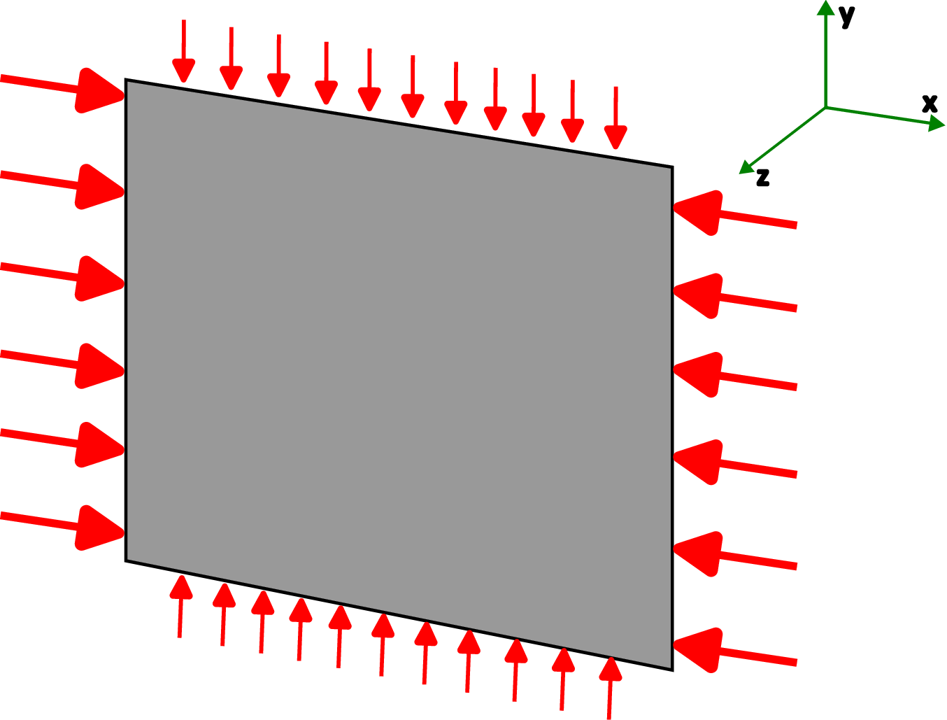
Solution: The
plane stress condition is used in analysis of thin plate-like structures. Here, strictly speaking, just the two \(z-\)faces (top
and bottom) of the structure are traction free due to which \(\sigma _{zz} = \tau _{xz} = \tau _{yz} = 0\) on just those two faces. However, the plate being thin in
\(z-\)direction, there is hardly any variation of \(\sigma _{zz}, \; \tau _{xz}, \; \tau _{yz}\) within the sample in its thickness direction. Hence \(\sigma _{zz} = \tau _{xz} = \tau _{yz} = 0\) is satisfied at every
point within the sample as well.
(a) To find \(\dfrac {\sigma _{xx}}{\epsilon _{xx}}\), we use the following stress-strain relation: \begin {align*} \begin {split} \epsilon _{xx}\;&=\;\dfrac {1}{E}\sbk {\sigma _{xx}\;-\;\nu \brc {\sigma _{yy}\;+\;\cancelto {0}{\sigma _{zz}}}}\\ \Rightarrow \frac {\epsilon _{xx}}{\sigma _{xx}} \; &=\;\dfrac {1}{E}\sbk {1\;-\;\nu \frac {\sigma _{yy}}{\sigma _{xx}} } \text {or}~\dfrac {\sigma _{xx}}{\epsilon _{xx}}\;=\;\dfrac {E}{\brc {1\;-\nu \alpha }}\quad \ldots \; (1) \end {split} \end {align*}
(b) To find the ratio of \(\epsilon _{xx}\) and \(\epsilon _{yy}\), we also need to determine \(\epsilon _{yy}\). Again using stress-strain relation: \begin {align*} \begin {split} \epsilon _{yy}\;=\;\dfrac {1}{E}\sbk {\sigma _{yy}\;-\;\nu \brc {\sigma _{xx}\;+\;\cancelto {0}{\sigma _{zz}}}} \Rightarrow \frac {\epsilon _{yy}}{\sigma _{xx}}\;=\;\dfrac {1}{E} \sbk {\alpha \;-\;\nu } \quad \ldots \; (2) \end {split} \end {align*}
Upon multiplying (1) and (2), we get the relation for \(\epsilon _{yy} /\epsilon _{xx}\): \begin {align*} \frac {\epsilon _{yy}}{\epsilon _{xx}}\;=\;\dfrac {\brc {\frac {\sigma _{yy}}{\sigma _{xx}}\;-\;\nu }}{\brc {1\;-\nu \frac {\sigma _{yy}}{\sigma _{xx}}}} =\; \dfrac {\brc {\alpha -\nu }}{\brc {1-\nu \alpha }}. \end {align*}
(c) \begin {align*} \begin {split} \epsilon _{zz}\;=\;\dfrac {1}{E}\sbk {\cancelto {0}{\sigma _{zz}}\;-\;\nu \brc {\sigma _{xx}\;+\;{\sigma _{yy}}}} \Rightarrow \frac {\epsilon _{zz}}{\sigma _{xx}}\;=\;-\dfrac {\nu }{E} \sbk {\frac {\sigma _{yy}}{\sigma _{xx}}\;+1} \quad \ldots \; (3) \end {split} \end {align*}
On multiplying (1) and (3), we get \begin {align*} \frac {\epsilon _{zz}}{\epsilon _{xx}}\;=\;-\nu \dfrac {\brc {\alpha \;+1}}{\brc {1\;-\nu \alpha }}. \end {align*}
Note that this ratio isn’t equal to negative of the Poisson’s ratio since it is not the case of uniaxial loading. On setting \(\alpha =0\) in order to mimic uniaxial loading scenario, we indeed see the ratio becoming \(-\nu \).
Solution:
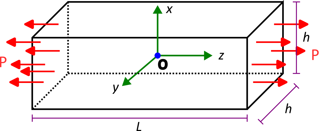
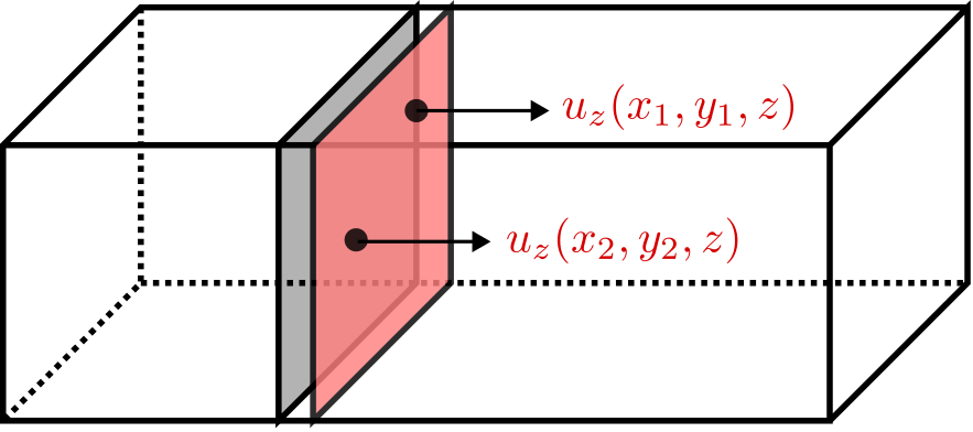
Plane cross-section remains plane even after deformation: It implies that all points in a given cross-section (which lies in \(x-y\) plane) of the beam must have the same \(u_z\), i.e., \(u_z(x_1, y_1, z) = u_z(x_2, y_2, z)\) (having different \(u_z\) at different \((x,y)\) points would lead to warping/bulging of the cross-section). Therefore, \(u_z\) must be independent of coordinates \(x\) and \(y\), i.e., \[u_z(x,y,z) = u_z(z).\]
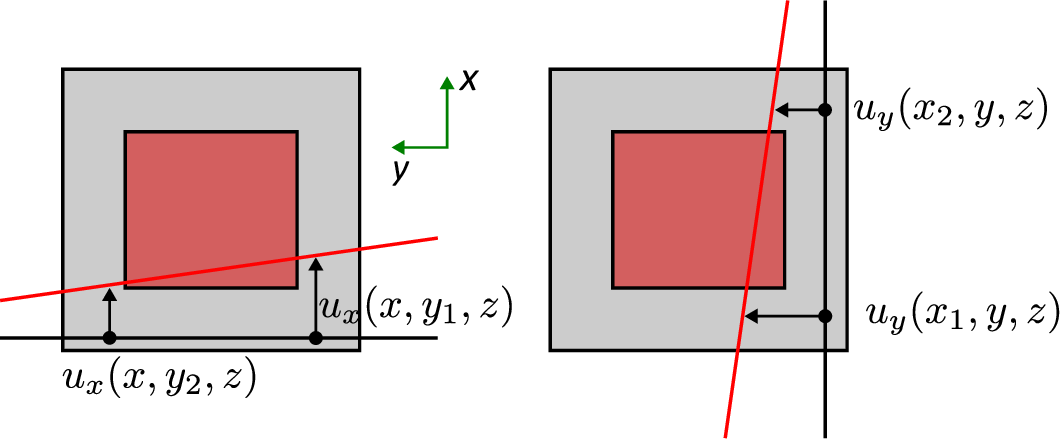
Cross-section remains square after deformation: It implies that in a cross-section, any horizontal (or vertical) line element must remain horizontal (or vertical) after deformation. From the following figure, it is clear that \(u_x\) for two different points having the same \(x-\)coordinate but different \(y-\)coordinates must have same \(u_x\) values after deformation, i.e. \(u_x(x,y_1,z) = u_x(x,y_2,z)\), to prevent tilting/curving of the line element connecting the two points. Thus \(u_x(x,y,z) = u_x(x,z)\). By a similar argument, \(u_y(x,y,z) = u_y(y,z)\).
Deformation is axially homogeneous: It implies that the beam cross-sections taken at different values of \(z\) along the axis of the beam will look the same. Physically, this implies the beam will deform uniformly along the axis of the beam as shown in the figure below:
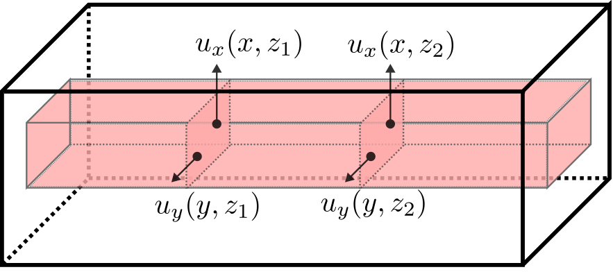
Alternatively, for any two cross-sections at \(z_1\) and \(z_2\), the displacements \(u_x(x,z_1)=u_x(x,z_2)\) and \(u_y(y,z_1)=u_y(y,z_2)\). Hence, we can say that \[u_x \text { and } u_y \text { are only functions of $x$ and $y$, respectively!}\]
Following similarly in \(y\) and \(z\) directions, we get \begin {align*} \dfrac {\partial ^2 u_{y}}{\partial y^2} &=0, \;\;\Rightarrow u_{y} = c y + d, \\ \dfrac {\partial ^2 u_{z}}{\partial z^2} &=0, \;\;\Rightarrow u_{z} = e y + f. \end {align*}
It is to be noted that since displacement components \(u_x,\;u_y,\;u_z \) are linear functions, the strain tensor \(\matr {\epsilon }\) will be constant, which also implies that stress tensor \(\matr {\sigma } = \matr {\matr {C}} \;\;\matr {\epsilon }\) will be constant throughout the beam (at all points).
On boundary conditions
The values of the constants \(a,b,c,d,e,f\) can be determined from displacement and traction boundary conditions.
Traction BC: We observe that \begin {align*} \sigma _{xx}|_{x=\pm h/2, y, z}\;&=\;0,\\ \sigma _{yy}|_{x, y=\pm h/2, z}\;&=\;0,\\ \sigma _{zz}|_{x, y, z=\pm L/2}\;&=\; \dfrac {P}{h^2}. \end {align*}
As we already know now that \(\matr {\sigma }\) is constant throughout the beam, it implies that \(\sigma _{xx}\;=\;\sigma _{yy}\;=\;0\) and \(\sigma _{zz} = \frac {P}{h^2}\) at every point in the beam.
To determine \(a\), \(c\) and \(e\), we substitute these values of \(\sigma _{xx}, \sigma _{yy}, \sigma _{zz}\) in stress-strain relations: \begin {align} \cancelto {0}{\sigma _{xx}}\;=\;\brc {\lambda \;+\;2\mu }\epsilon _{xx}\;+\;\lambda \brc {\epsilon _{yy}\;+\;\epsilon _{zz}} \Rightarrow \; \brc {\lambda \;+\;2\mu }a\;+\;\lambda \brc {c\;+\;e}=\;0,\notag \\ \cancelto {0}{\sigma _{yy}}\;=\;\brc {\lambda \;+\;2\mu }\epsilon _{yy}\;+\;\lambda \brc {\epsilon _{xx}\;+\;\epsilon _{zz}} \Rightarrow \; \brc {\lambda \;+\;2\mu }c\;+\;\lambda \brc {a\;+\;e}=\;0,\notag \\ \cancelto {\frac {P}{h^2}}{\sigma _{zz}}\;=\;\brc {\lambda \;+\;2\mu }\epsilon _{zz}\;+\;\lambda \brc {\epsilon _{xx}\;+\;\epsilon _{yy}} \Rightarrow \brc {\lambda \;+\;2\mu }e\;+\;\lambda \brc {a\;+\;c}\;=\;\dfrac {P}{h^2} .\notag \end {align}
Solving the above three equations, we get the constants \(a,c,e\) and finally obtain the displacement components (\(u_x, u_y, u_z\)). For example, upon subtracting first two equations, we get \(a=c\) which when substituted into the first equation leads to \begin {equation*} a=c=-\frac {\lambda }{2(\lambda +\mu )}e = -\nu ~e. \end {equation*} This simply implies that the ratio of lateral strain and longitudinal strain during uniaxial loading equals negative of the Poisson’s ratio. Note that the constants \((a,c,e)\) are the normal strains along three directions in this case.
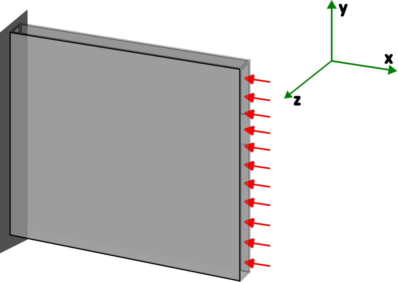
Solution: In this problem, the out-of-plane displacement along \(z\) is zero, i.e., \(u_z\;=\;0\). Furthermore \(u_x\;=\;u_x\brc {x,y}\) and \(u_y\;=\;u_y\brc {x,y}\).
Observe that all non-zero strain components are confined in \(x-y\) plane: this condition represents plane-strain condition. All the strain components associated with out-of-plane direction are zero, i.e., \[\epsilon _{zz}\;=\;0\] \[\gamma _{xz}\;=\;\dfrac {\partial u_x}{\partial z}\;+\;\dfrac {\partial u_z}{\partial x}\;=\;0\] \[\gamma _{yz}\;=\;\dfrac {\partial u_y}{\partial z}\;+\;\dfrac {\partial u_z}{\partial y}\;=\;0\] Using stress-strain relation for isotropic materials, we could write the stress matrix as follows: \begin {align*} \sbk {\matr {\sigma }} = \begin {bmatrix} \sigma _{xx} & \tau _{xy} & 0\\ \tau _{xy} & \sigma _{yy} & 0\\ 0 & 0 & \sigma _{zz} \end {bmatrix} = \begin {bmatrix} (\lambda + 2 \mu ) \epsilon _{xx} + \lambda \epsilon _{yy} & 2\mu \epsilon _{xy} & 0\\ 2\mu \epsilon _{xy} & (\lambda + 2 \mu ) \epsilon _{yy} + \lambda \epsilon _{xx} & 0\\ 0 & 0 & \lambda \brc {\epsilon _{xx} + \epsilon _{yy}} \end {bmatrix}. \end {align*}
Note that \(\sigma _{zz}\) is not zero since as the plate is being compressed along \(-x\) direction, it will try to expand in \(y\) and \(z\) directions. However, out-of-plane displacement is not allowed (\(u_z=0\)) which means some constraint is preventing expansion along \(z\) and, in turn, the constraint applies a non-zero compressive stress \(\sigma _{zz}\) on the plate’s \(z-\)faces.
Here \(\dfrac {\partial \brc {\epsilon _{xx} + \epsilon _{yy}}}{\partial z} = 0\) because \(\epsilon _{xx}\) and \(\epsilon _{yy}\) are not functions of \(z\). So the stress-equilibrium equation for \(z-\)direction is automatically satisfied for plane strain condition.
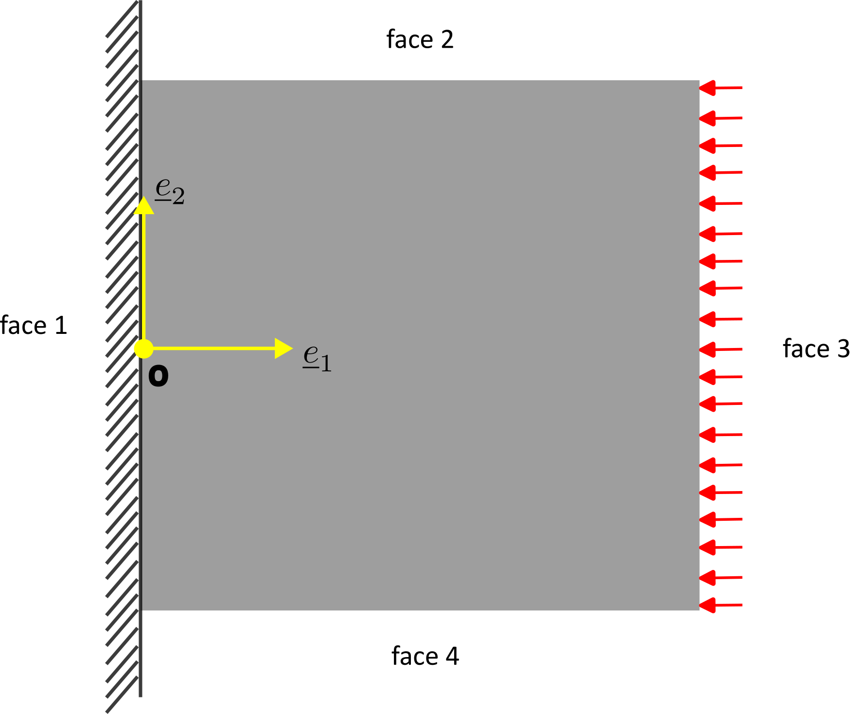
The displacement and traction boundary conditions that will be used to solve this problem are as follows:
Displacement BC on face 1: \[u_x \mid _{(0,y)} = u_y \mid _{(0,y)} = 0. \]
Traction BC on face 2: \[\matr {\sigma }~\ve {e}_2 |_{\text {face 2}}\;=\;\begin {bmatrix} \tau _{xy}\\ \sigma _{yy} \\ \sigma _{zy} \end {bmatrix}\;=\;\begin {bmatrix} 0\\ 0\\ 0 \end {bmatrix}.\]
Traction BC on face 3: \[\matr {\sigma }~\ve {e}_1 |_{\text {face 3}}\;=\;\begin {bmatrix} \sigma _{xx}\\ \tau _{xy} \\ \tau _{xz} \end {bmatrix}\;=\;\begin {bmatrix} -p\\ 0\\ 0 \end {bmatrix}.\]
Traction BC on face 4: \[\matr {\sigma }~ -\ve {e}_2 |_{\text {face 4}}\;=\;\begin {bmatrix} -\tau _{xy}\\ -\sigma _{yy} \\ -\sigma _{zy} \end {bmatrix}\;=\;\begin {bmatrix} 0\\ 0\\ 0 \end {bmatrix}.\]
or \begin {align} &\epsilon _{11} = \frac {1}{E}(\sigma _{11}-\nu (\sigma _{22}+\sigma _{33})),~\epsilon _{22} = ...,~\epsilon _{33} = ....\nonumber \\ &\gamma _{12} = \tau _{12}/G,~\gamma _{23} = ...,~\gamma _{13}=...\nonumber \end {align}
Using the above two equivalent approaches, express \((E,G,\nu )\) in terms of \((\lambda ,\mu )\).
Solution: The two formulations can be written as follows in a matrix form: \begin {align} \begin {bmatrix} \sigma _{11} \\ \sigma _{22} \\ \sigma _{33} \end {bmatrix} \;=\; \begin {bmatrix} \gamma \;+\;2\mu & \gamma & \gamma \\ \gamma & \gamma \;+\;2\mu & \gamma \\ \gamma & \gamma & \gamma \;+\;2\mu \end {bmatrix}\begin {bmatrix} \epsilon _{11} \\ \epsilon _{22} \\ \epsilon _{33} \end {bmatrix} \nonumber \end {align}
or \begin {align} \begin {bmatrix} \epsilon _{11} \\ \epsilon _{22} \\ \epsilon _{33} \end {bmatrix} \;=\; \dfrac {1}{E}\begin {bmatrix} 1 & -\nu & -\nu \\ -\nu & 1 & -\nu \\ -\nu & -\nu & 1 \end {bmatrix}\begin {bmatrix} \sigma _{11} \\ \sigma _{22} \\ \sigma _{33} \end {bmatrix}. \nonumber \end {align}
Taking the inverse of first matrix equation and equating to second matrix equation will give the desired relations \(E\brc {\gamma ,\;\mu },\;\nu \brc {\gamma ,\;\mu }\). Also note that \begin {align} \sigma _{12}\;=\;2\mu \epsilon _{12}\;=\;\mu \gamma _{12}\quad \text {(using first approach)},\nonumber \\ \gamma _{12}\;=\;\dfrac {\tau _{12}}{G} \quad \text {(using second approach)}.\nonumber \end {align}
On comparing, we get \(\mu \;=\;G \).
Alternative approach
We know \(E\;=\;\dfrac {\sigma _{11}}{\epsilon _{11}}\) and \(\nu \;=\;-\dfrac {\epsilon _{22}}{\epsilon _{11}}\;=\;-\dfrac {\epsilon _{33}}{\epsilon _{11}} \) from unixial loading. Let us substitute this special case in the below general equation: \begin {align} \label {eq: 1.6} \sigma _{ij}\;=\;\lambda \; tr\brc {\matr {E}} \delta _{ij} \;+\;2 \mu \epsilon _{ij}. \end {align}
For \(i\;=\;j\;=\;1\), we get \begin {align} \sigma _{11}\;&=\;\brc {\lambda \;+\;2\mu }\epsilon _{11}\;+\;\lambda \brc {\epsilon _{22}\;+\;\epsilon _{33}}\notag \\ \Rightarrow \; E\epsilon _{11}\;&=\;\brc {\lambda \;+\;2\mu }\epsilon _{11}\;-\;2\lambda \nu \epsilon _{11} \Rightarrow \;E\;=\;\brc {\lambda \;+\;2\mu }\;-\;2\lambda \nu . \nonumber \end {align}
For \(i\;=\;j\;=\;2\), \begin {align} \sigma _{22}\;&=\;\brc {\lambda \;+\;2\mu }\epsilon _{22}\;+\;\lambda \brc {\epsilon _{11}\;+\;\epsilon _{33}} \notag \\ \Rightarrow \;0\;&=\;-\brc {\lambda \;+\;2\mu }\nu \epsilon _{11}\;+\;\lambda \brc {1\;-\;\nu }\epsilon _{11} \Rightarrow \; \nu \;=\;\dfrac {\lambda }{2\brc {\lambda \;+\;\mu }}. \nonumber \end {align}
On substituting \(\nu \) from the above case into first case, we get \begin {align*} E =\lambda \;+\;2\mu \;-\;2\lambda \;\dfrac {\lambda }{2\brc {\lambda \;+\;\mu }} =\dfrac {\lambda ^2\;+\;3\lambda \mu \;+\;2\mu ^2\;-\;\lambda ^2}{\brc {\lambda \;+\mu }} =\dfrac {\mu \brc {3\lambda \;+\;2\mu }}{\lambda \;+\;\mu }. \end {align*}
X is an example of
The number of independent material constants for the material X is
\(u_x = ay\), \(u_y = 0\), \(u_z = 0\)
This is also called simple shearing of a body. Here \(a\) is a constant denoting the amount of shear. Assuming the body were isotropic, which component of stress would be non-zero?
\(u_x = ay\), \(u_y = 0\), \(u_z = 0\)
This is also called simple shearing of a body. Here \(a\) is a constant denoting the amount of shear. What is the value of maximum principal stress (assume shear modulus is ‘G’)?
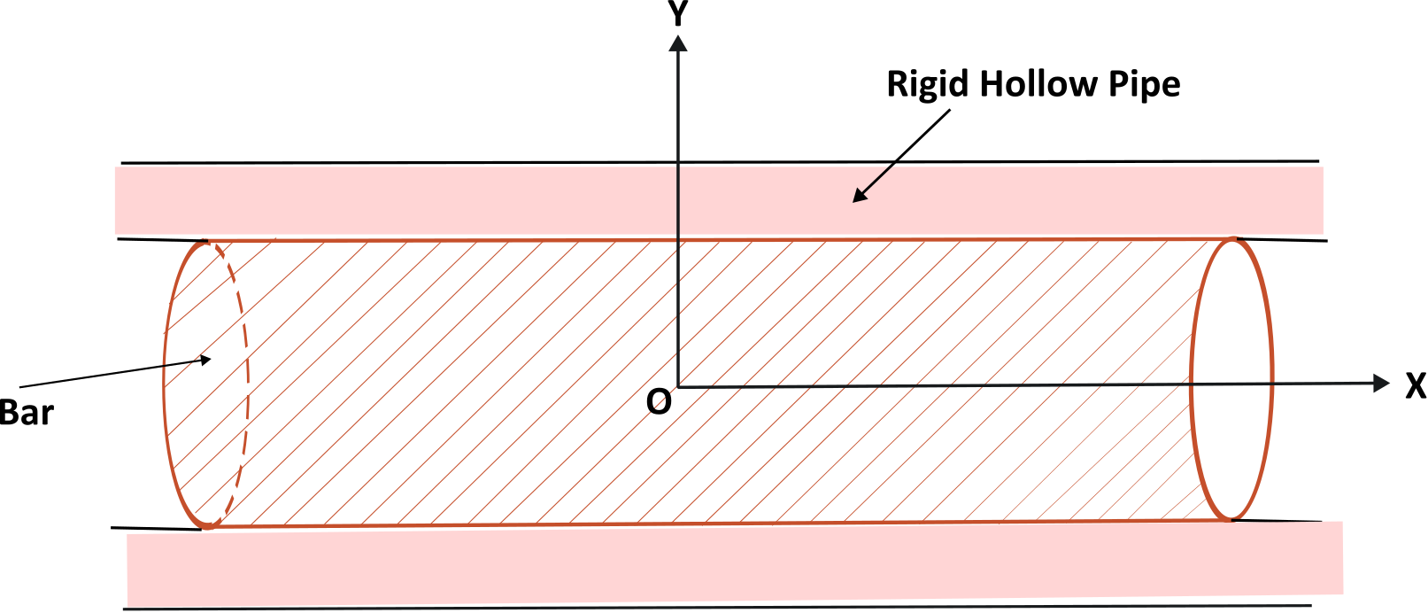
What can you say about strain induced in the body?
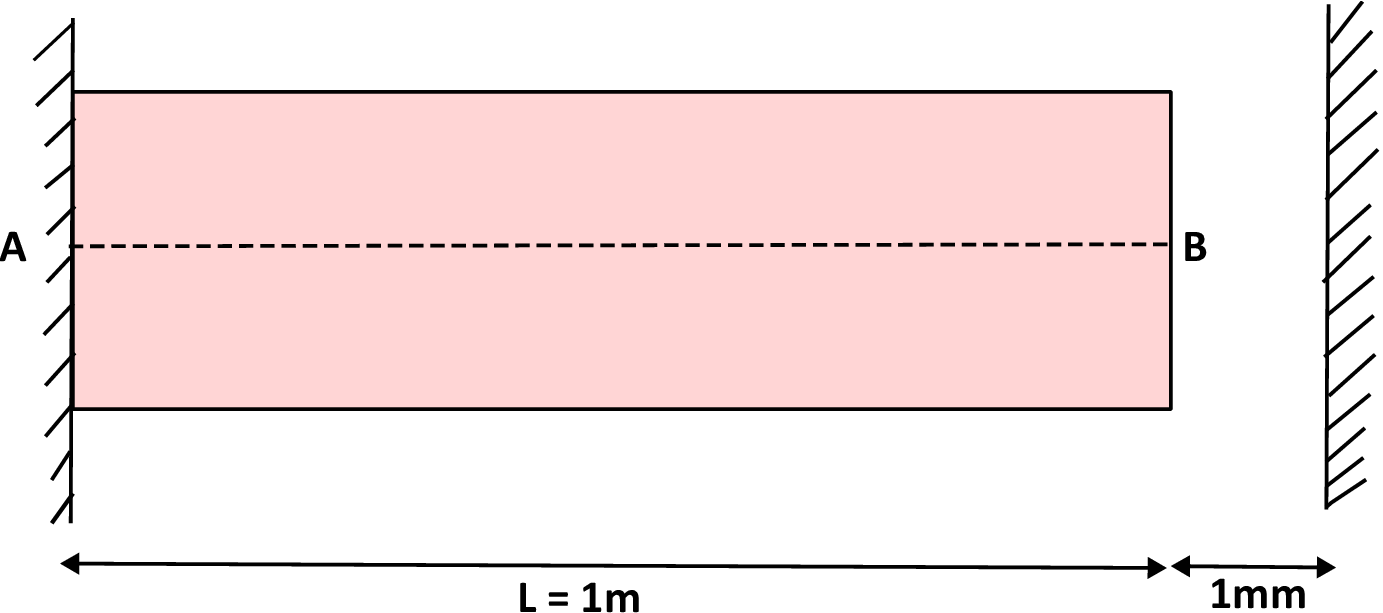
The stress components in terms of Poisson’s ratio (\(\nu \)), coefficient of thermal expansion (\(\alpha \)) and temperature change (\(T_0\)) will be
What can you say about shear stress components?
∗When quantities are expressed in terms of current position of a particle, it is called Eulerian description which is commonly used in Fluid mechanics. In Eulerian description, expression for acceleration becomes a bit complicated.
†Often, this stress-strain relation is also called constitutive relation.
‡The reference configuration of the body is also its zero strain state.
§A rigorous approach is to also account for symmetry of strain components in the derivative calculation \eqref{6_strain_der} which we have ignored for simplicity.
¶This is a generalized Hooke’s law for three-dimensional deformation of a body as compared to one-dimensional Hooke’s law (\(\sigma =E\epsilon \)) which relates stress and strain for the axial deformation of a bar.