In this chapter, we will learn a new topic Energy Methods which is an alternate method to obtain deformation of general structures including beams. Unlike stress equilibrium equations solving which we obtain displacement of every point in a body simultaneously, the energy methods gives displacement of only few special points in the body. However, as we will see, the new approach is algebraic in nature and much simpler to solve than partial differential equations. We will first learn about various concepts needed for understanding energy methods. We will then see how one can apply this method for solving beam deformation problems.
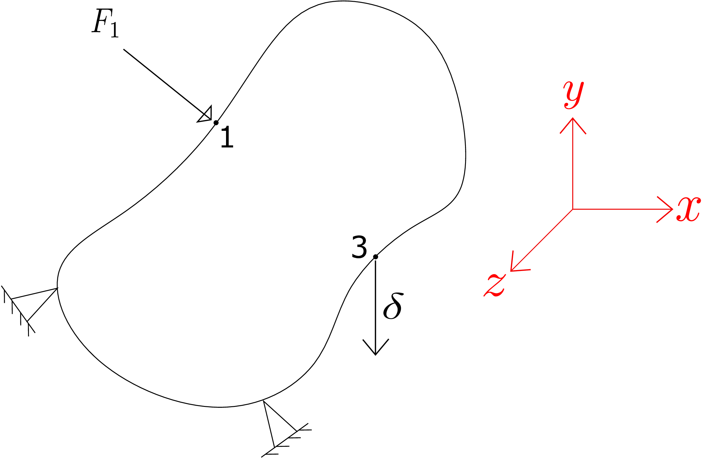
Consider an arbitrary body as shown in Figure 10.1.
It is clamped at two points and subjected to a concentrated load \(F_1\) at point 1. Let us say we want to measure the deflection \(\delta \) at a different point (say point 3 in the figure) which can be either on the surface of the body or within the body. How is the deflection \(\delta \) related to force \(F_1\)? To explore it, let us look at the stress equilibrium equations as given below:
These equations are supplemented with the following boundary conditions:
Notice that the above equations are linear in stress components which, in turn, are linear in strain components (due to linear stress-strain relation). Finally, strain components are also linear in displacement components.∗ Thus, the governing equations become linear in unknown displacement components. Similarly, the boundary conditions are also linear in unknown displacement components. Due to this linearity of governing equations, the displacement of the body will be linearly related to externally applied load. In fact, this linearity also allows superposition principle to hold. The external load here consists of the body force and boundary traction/point loads. Coming back to the problem shown in Figure 10.1, \(\delta _3\) will thus be linearly related to the applied load \(F_1\), i.e.,
The proportionality constant \(k_{31}\) is also called influence coefficient. If we change the point of location of force \(F_1\), \(k_{31}\) will change. Similarly, if we change the point at which we are measuring the displacement, \(k_{31}\) will change. Hence, the influence coefficient depends on the location of the applied force as well as on the location of the point where displacement is being measured. In fact, it also depends on the direction of applied force and the direction in which displacement is being measured but does not depend on the magnitude of force. For example, displacement being a vector quantity, \(\underline {\delta }_3\) will have three components \(\delta _3^x\), \(\delta _3^y\) and \(\delta _3^z\). For each of the components, we will have different influence coefficients relating to each component of force applied at point 1, i.e.,
Each of the equations above resembles Hooke’s law for a spring where force in the spring is proportional to the elongation in the spring. The above equations hold only if just one (but any) of the components of force is acting at a time. In case all components are present simultaneously, one can apply the principle of superposition as mentioned earlier which would yield
Note that the influence coefficients are unaffected whether only one component of force is present or all the components are present. The principle of superposition would hold similarly even if the force is acting at two (or more) different points in the body. For example, suppose we only apply a force \(F_1\) at point 1 and no other force, the displacement at point 3 in a prescribed direction will be given by \begin {equation} \delta _3=k_{31}F_1. \end {equation} In another situation, if we apply a force \(F_2\) at point 2 and no other force, the displacement at point 3 in the same direction will be given by \begin {equation} \delta _3=k_{32}F_2. \end {equation} In a third situation, if we apply force \(F_1\) at point 1 and force \(F_2\) at point 2 together, the displacement at point 3 (again in the same direction) will be \begin {equation} \delta _3=k_{31}F_1+k_{32}F_2. \end {equation} Notice that the influence coefficients are the same as in the case when only one of the forces were acting.
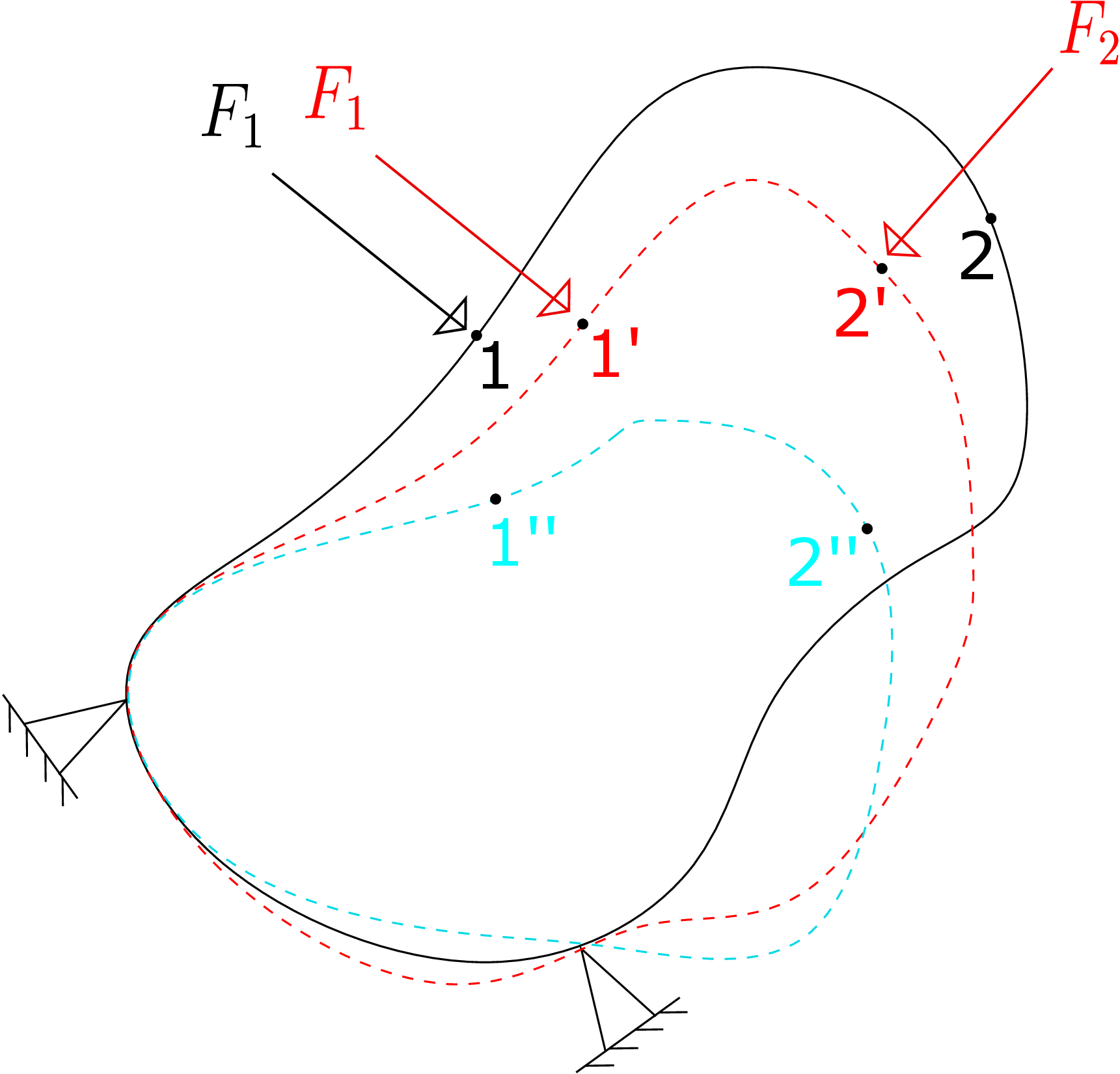
Consider an arbitrary body clamped at two locations. We apply a force \(F_1\) at point 1 and measure vertical component of displacement at point 3 (see Figure 10.2a).
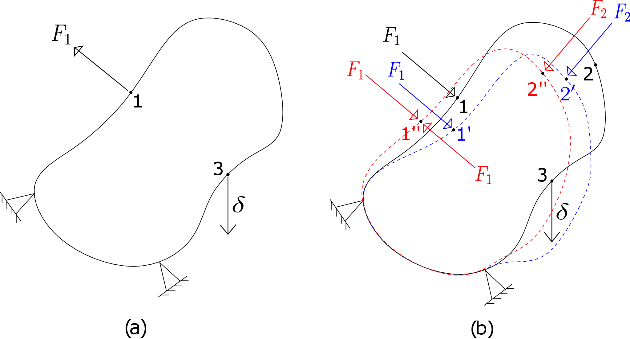
The displacement will be \begin {equation} \delta _3=k_{31}F_1. \end {equation} Due to the application of force, the system must have deformed and changed its shape and size (see blue dotted lines in Figure 10.2b). In the next step, we apply force \(F_2\) at point 2’ (originally at 2) in the deformed body. So, both \(F_1\) and \(F_2\) are acting now. As \(F_2\) is applied after the body has deformed, the influence coefficient \(k_{32}\) may have changed to \(k_{32}'\) which implies \begin {equation} \label {step2} \delta _3=k_{31}F_1+k'_{32}F_2. \end {equation} In the third step, we apply a force \(-F_1\) at point 1” (originally at 1) in the current deformed body (see Figure 10.2b). Due to this, the total force acting at point 1 becomes zero and we are only left with a force \(F_2\) at point 2” (originally at 2). As the condition of the body has changed, the influence coefficient \(k_{31}\) may have changed to \(k''_{31}\). So, the total vertical displacement at the same point 3 will be \begin {equation} \label {10_three_step} \delta _3=k_{31}F_1+k'_{32}F_2+k''_{31}(-F_1). \end {equation} Alternately, as in the final configuration, we only have a force \(F_2\) at point 2, the vertical displacement of point 3 should be \begin {equation} \label {10_one_step} \delta _3=k_{32}F_2. \end {equation} Notice that we have used the original influence coefficient in the above equation as if only force \(F_2\) were acting right from the beginning. We could say so because the displacement in an elastic body only depends on the final state of applied load and does not depend on how those loads were applied. Equating equations \eqref{10_three_step} and \eqref{10_one_step} since the final state of loading is the same, we obtain
Since this has to hold for arbitrary magnitudes of (\(F_1,F_2\)), their coefficients must vanish. Thus, we get
This means that in step 2 when both \(F_1\) and \(F_2\) act, the displacement would simply be \begin {equation} \delta _3=k_{31}F_1+k_{32}F_2 \end {equation} which proves that one can apply superposition principle.
The displacement of the body at the point of application of force and in the same direction as the applied force is called the corresponding displacement. As this component of displacement is also responsible for the actual work done by the force, it is therefore also called the work absorbing displacement. Suppose we apply force at point 1 and measure the corresponding displacement \(\delta _1\), then
We now want to find the energy stored in a deformable body due to a force, say \(F_1\). Would it simply be \(F_1\delta _1\) where \(\delta _1\) is the corresponding displacement. To find an answer to this, consider a spring having spring constant \(k\) and clamped at one end. A force \(F\) is applied at its other end as shown in Figure 10.3a.
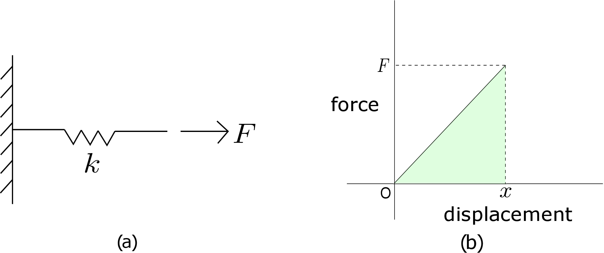
We know that the energy stored in the spring due to this force is
Here \(x\) denotes the elongation in the spring or the displacement of other end which is also the corresponding
displacement. To understand the origin of the factor \(\frac {1}{2}\) in the above expression, we can think of pulling the spring very
slowly. When the displacement of the spring is \(\Delta \), the force within the spring is just \(k\Delta \). So, to ramp up the displacement
from 0 to \(x\), we need to ramp up the force from 0 to \(kx\) (\(=F\)). The corresponding force-displacement curve
is shown in Figure 10.3b. The work done in this quasistatic process will be the area of the shaded
triangle (\(=\frac {1}{2}F\cdot x\)). However, the final energy stored in an elastic system is independent of the loading path
taken in the process: it only depends on the final force/displacement. Thus, even if we apply the force
instantly to reach the final stage, the energy stored would still be \(\frac {1}{2}F x\) although the work done by the
external agent is \(F x\). The other half of the energy either gets converted into kinetic energy or dissipates as
heat.†
Taking the analogue of spring, we can now note that the energy stored in a deformable body due to the action of
force \(F_1\) would be
This is the energy stored due to a single force. We can have multiple forces \(F_1,F_2,...F_n\) (with corresponding displacements \(\delta _1,\delta _2,...\delta _n\)) acting on the deformable body as shown in Figure 10.4.
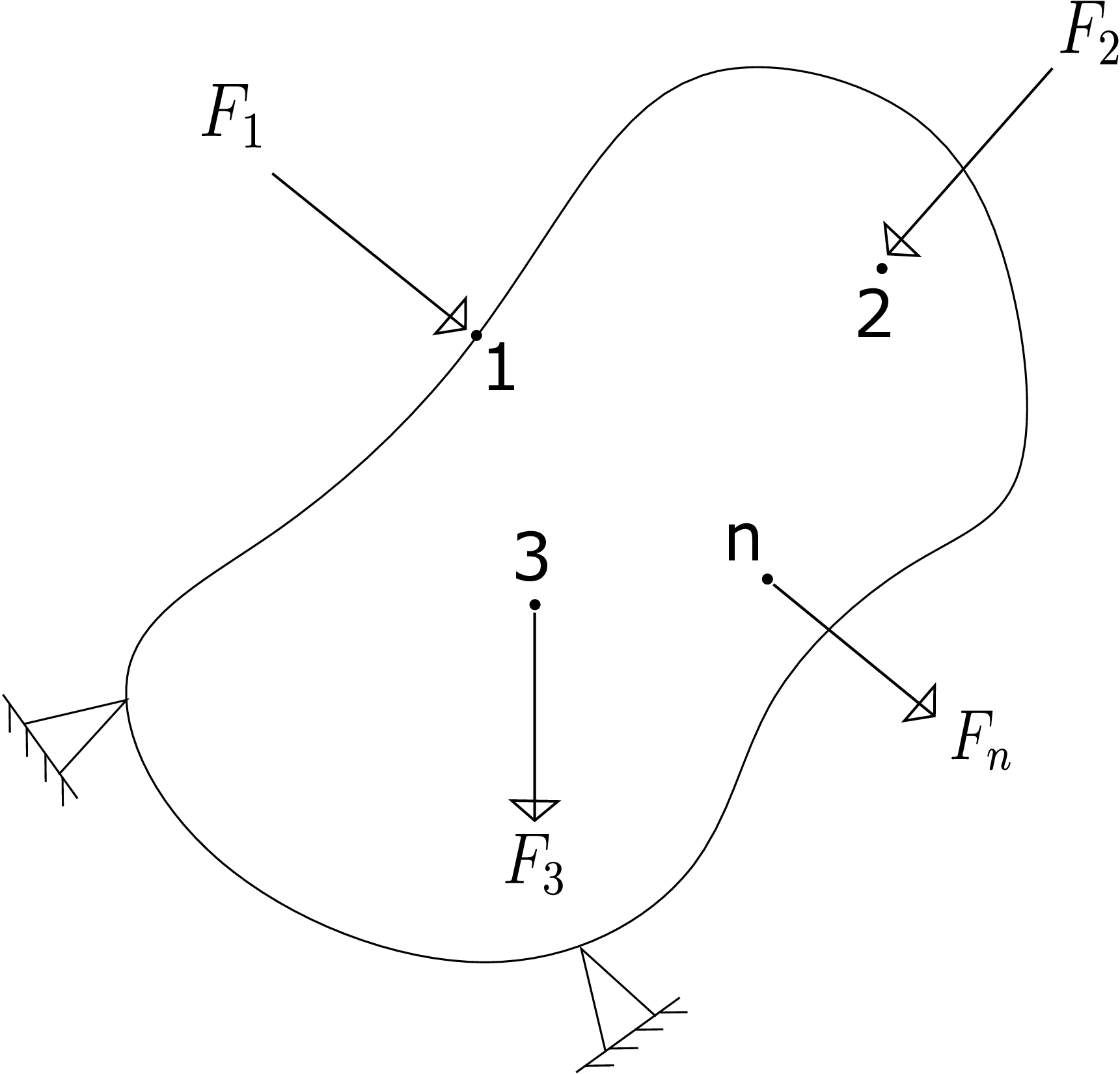
The total energy stored would be \begin {equation} \label {10_energy1} \sum _{i=1}^n\frac {1}{2}F_i\delta _i. \end {equation} In the above, we cannot substitute \(\delta _i\) as \(k_{ii}F_i\) because \(\delta _i\) contains contributions from multiple forces. It would be the following: \begin {equation} \delta _i=\sum _{i=1}^nk_{ij}F_j. \end {equation} Plugging this into equation \eqref{10_energy1}, we get \begin {equation} \text {Total energy stored}=\sum _{i}\sum _j\frac {1}{2}k_{ij}F_i F_j. \end {equation} This is the expression of total energy stored in the body in terms of the applied forces and influence coefficients.
The reciprocal relation allows us to obtain a relationship between influence coefficients \(k_{ij}\) and \(k_{ji}\). Let us work this out through energy considerations. We will consider two different processes. In the first process, think of a body with a force \(F_1\) applied on it at point 1. The energy stored in the body will be \begin {equation} E=\frac {1}{2}F_1\delta _1=\frac {1}{2}F_1 ~(k_{11}F_1)=\frac {1}{2}k_{11}F_1^2. \end {equation} This action is shown in Figure 10.5 where due to this force, the body deforms from solid black configuration to the dashed red configuration. We call this step 1 where the point 1 gets displaced to 1’ during deformation.
Then, we apply force \(F_2\) at point 2’ in the current configuration which was at point 2 in the original/undeformed body. The body gets further deformed to the dashed blue configuration as shown in Figure 10.5. The point 1’ goes to 1” and 2’ goes to 2”. This is step 2. The energy stored in the body in the final state will be
Notice that the contribution to energy due to \(F_1\) during step 2 is not divided by 2. This is because during step two, the
full \(F_1\) acts throughout the deformation: the work done will thus simply be the force \(F_1\) times the extra displacement (\(1'\to 1''\)).
This additional displacement is nothing but the displacement due to \(F_2\), i.e., \(k_{12}F_2\). The work done due to the sudden
application of force \(F_2\) is the same as the ramped up work. Thus, it is divided by 2. The corresponding displacement in
this term represents movement of 2’\(\to \)2” (and not of 2\(\to \)2”) as this part of displacement is the one due to the application
of \(F_2\) which can be written as \(k_{22}F_2\).
We now think of the second process which is basically the first process only but the order of the two steps are
reversed here. This means that we first apply force \(F_2\) and then apply force \(F_1\) in the second step. Due to application of \(F_2\)
in the first step, the energy stored in the body will be \begin {equation} E=\frac {1}{2}k_{22}F_2^2. \end {equation} In the second step, \(F_1\) is applied. As \(F_2\) is acting fully in this step,
the additional energy due to it in step 2 will not be divided by 2. The total energy stored in the body will thus be
Now, in both the processes, the final state is the same with both \(F_1\) and \(F_2\) acting. Thus, the final energy stored in the two processes must be the same. Hence, upon comparing equations \eqref{10_energy_process1} and \eqref{10_energy_process2}, we get \begin {equation} k_{12}=k_{21}. \end {equation} Generalizing this, we can write the reciprocal relation as \begin {equation} k_{ij}=k_{ji}. \end {equation}
Consider again a body which is clamped at some points. We think of two situations. In the first situation, multiple forces \(F_1,F_2,...F_n\) are applied on it as shown in Figure 10.4. The corresponding displacements for these forces are \(\delta _1,\delta _2,...\delta _n\). In the second situation, we apply forces \(F_1',F_2',...F_n'\) each at the same location and direction but of different magnitude. We further measure the corresponding displacements \(\delta _1',\delta _2',...\delta _n'\). The Maxwell-Betti-Rayleigh reciprocal theorem tells us that \begin {equation} \label {10_reciprocal_theorem} \sum _{i=1}^nF_i\delta '_i=\sum _{i=1}^nF'_i\delta _i. \end {equation} This means that the work done by forces in situation 1 through the corresponding displacements of situation 2 equals the work done by forces in situation 2 through the corresponding displacements of situation 1. Let us try to prove this. Consider the LHS of equation \eqref{10_reciprocal_theorem}:
We can rearrange these terms by collecting the first terms within each bracket, second terms within each bracket and so on, i.e.,
This completes the proof of reciprocal theorem.
Till now, we have only discussed about forces and displacements. The above relations can be extended to moments and rotations as well. Just like the work analog of force is displacement, the work analog of moment is rotation. Consider an arbitrary body on which several forces and moments act (see Figure 10.6).
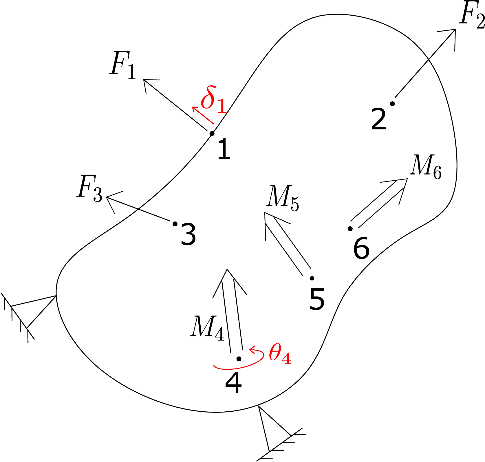
We can measure the corresponding displacements and corresponding rotations. A corresponding rotation is the local rotation of the deformable body in the direction of the applied moment at the same point. Moments and rotations can be seen as generalized forces and generalized displacements, respectively. If we think in these terms, all the relations derived earlier do not differentiate between forces and moments or between displacements and rotations. Thus, all the earlier relations will hold for moments and rotations also. For example, the corresponding rotation \(\theta _4\) for \(M_4\) will be given by \begin {equation} \theta _4=k_{41}F_1+k_{42}F_2+k_{43}F_3+k_{44}M_4+k_{45}M_5+k_{46}M_6. \end {equation} The dimensions of the influence coefficients relating force and rotation and those relating moment and rotation are different though. For example, the dimension of \(k_{41}\) is \(\frac {\theta }{force}\) or \(\frac {1}{force}\) while that of \(k_{44}\) is \(\frac {\theta }{moment}\) or \(\frac {1}{moment}\).‡ Similarly, the corresponding displacement for force \(F_1\) can be written as \begin {equation} \delta _1=k_{11}F_1+k_{12}F_2+k_{13}F_3+k_{14}M_4+k_{15}M_5+k_{16}M_6. \end {equation} The dimension of \(k_{11}\) is \(\frac {displacement}{force}\) while that of \(k_{14}\) is \(\frac {displacement}{moment}\). As the dimension of moment equals that of force times displacement, the dimension of \(k_{14}\) can also be written as that of \(\frac {1}{force}\). This means that the dimensions of \(k_{14}\) and \(k_{41}\) are the same. So, the reciprocal relation can also be easily extended to mixed combinations (i.e., displacement-moment or rotation-force) and one can write \begin {equation} k_{14}=k_{41} \end {equation} as earlier.
We have already derived the expression for energy stored in a deformable body as \begin {equation} E=\sum _i\frac {1}{2}F_i\delta _i=\sum _i\frac {1}{2}F_i\bigg (\sum _jk_{ij}F_j\bigg )=\sum _i\sum _j\frac {1}{2}k_{ij}F_iF_j. \end {equation} Let us take the first derivative of this expression with respect to the \(k\)th generalized force:
Upon further replacing the summation index \(j\) with \(i\), we get
We have thus derived that the corresponding displacement \(\delta _k\) is the derivative of total energy with respect to the corresponding force \(F_k\). This is called the Castigliano’s first theorem. If we can write the total energy stored in a body in terms of the applied forces/moments, we can apply this theorem to find the corresponding displacement/rotation. We need not solve any differential equation. Of course, we need to know all the influence coefficients.
Writing the stored energy in terms of externally applied generalized forces is crucial if we want to use the Castigliano’s first theorem. Let us see how this can be achieved. Think of a general three-dimensional body which is clamped at some points as shown in Figure 10.7a.
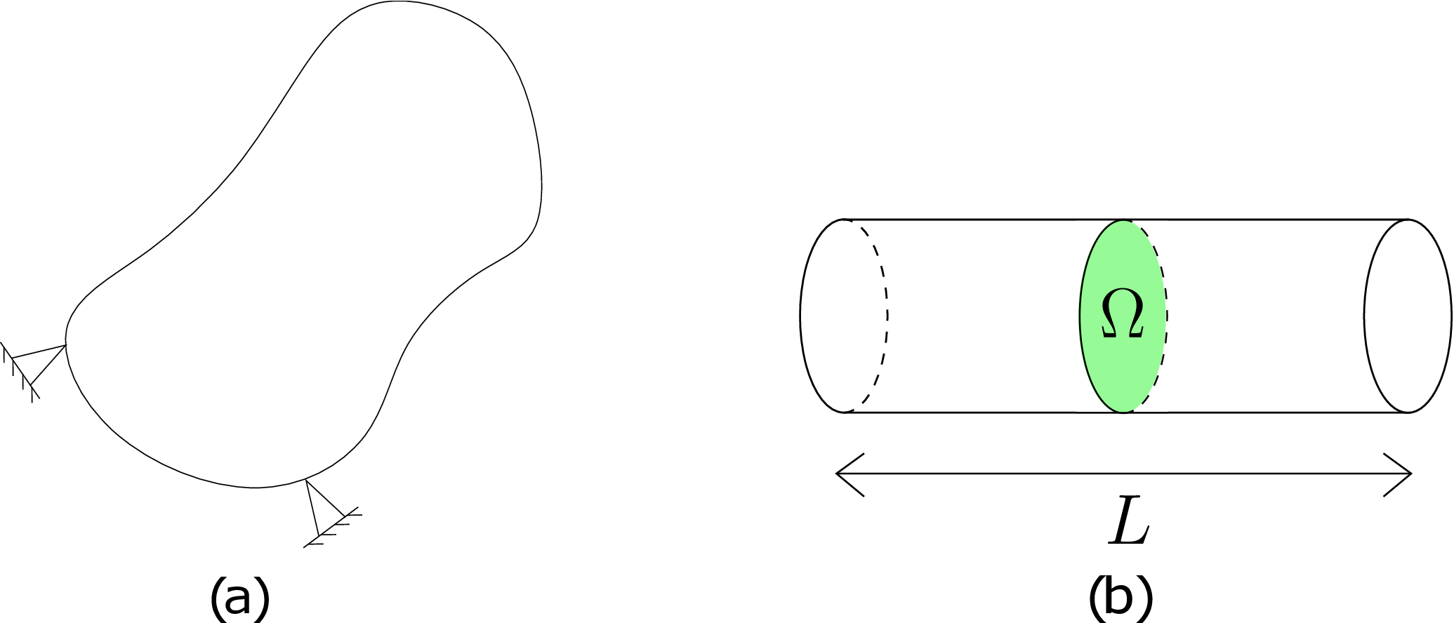
We want to know the energy stored in this body. For linear stress-strain relation, the energy stored becomes \begin {equation} \label {10_energy_general} E=\sum _i\sum _j\iiint _V\frac {1}{2}\sigma _{ij}\epsilon _{ij}dV. \end {equation} Let us simplify this further in the context of beams which we will be mostly dealing with. Consider the beam shown in Figure 10.7b having cross-section \(\Omega \) and length \(L\). The equation \eqref{10_energy_general} can be rewritten as follows for a beam: \begin {equation} \label {energy_beams} E=\int _0^Lds\bigg (\sum _i\sum _j\iint _\Omega \frac {1}{2}\sigma _{ij}\epsilon _{ij}\,d\Omega \bigg ) \end {equation} We will call the integral in the parentheses above the cross-sectional strain energy as it is obtained by integration of the three-dimensional strain energy density over the beam’s cross-section. It is further integrated over the length of the beam to obtain the total energy stored in a beam. A beam can deform in several modes such as bending, twisting, stretching and shearing. For each of these deformation modes, the energy stored in the beam’s cross-section has different mathematical form. Let’s discuss them one by one.
Consider a beam being stretched by the application of an axial load \(P\) as shown in Figure 10.8.
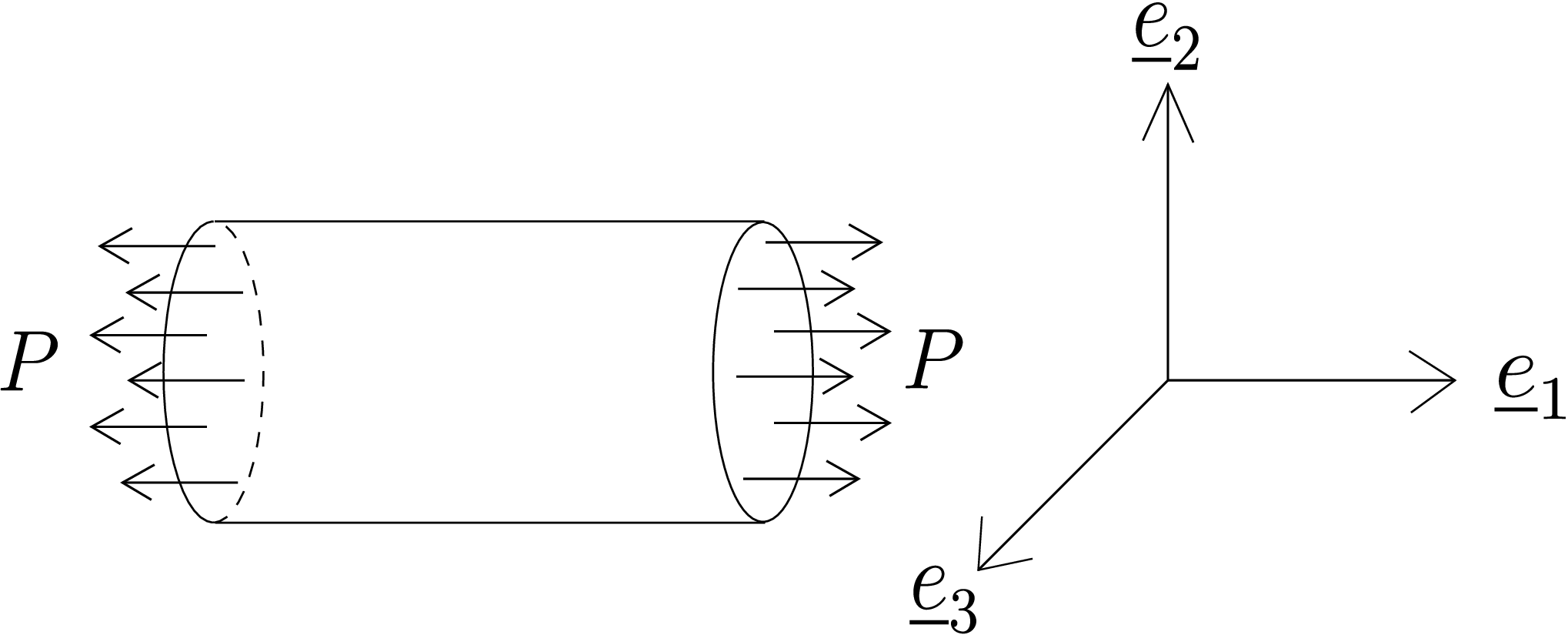
The total load \(P\) can be assumed to be uniformly distributed over the cross-section \(\Omega \). To find the energy stored in the cross-section, we need to first find the stress and strain components. We can recall from earlier discussion that in case of axial extension of a beam, the cross-section is allowed to relax freely. So, the stress matrix has only one non-zero stress component, i.e., \begin {equation} \begin {bmatrix}\underline {\underline {\sigma }}\end {bmatrix}= \begin {bmatrix} \sigma _{11} & 0 & 0\\ 0 & 0 & 0\\ 0 & 0 & 0 \end {bmatrix}. \end {equation} Using three-dimensional Hooke’s Law, we can then write
The cross-sectional energy will thus become
In the last step, we assumed that the axial load \(P\) is uniformly distributed over the cross-section. Upon final integration over the cross-section, we get
This can be further integrated over the length of the beam to get the total energy due to stretching of a beam.
Figure 10.9 shows a beam which bends due to the application of bending moment \(M\).
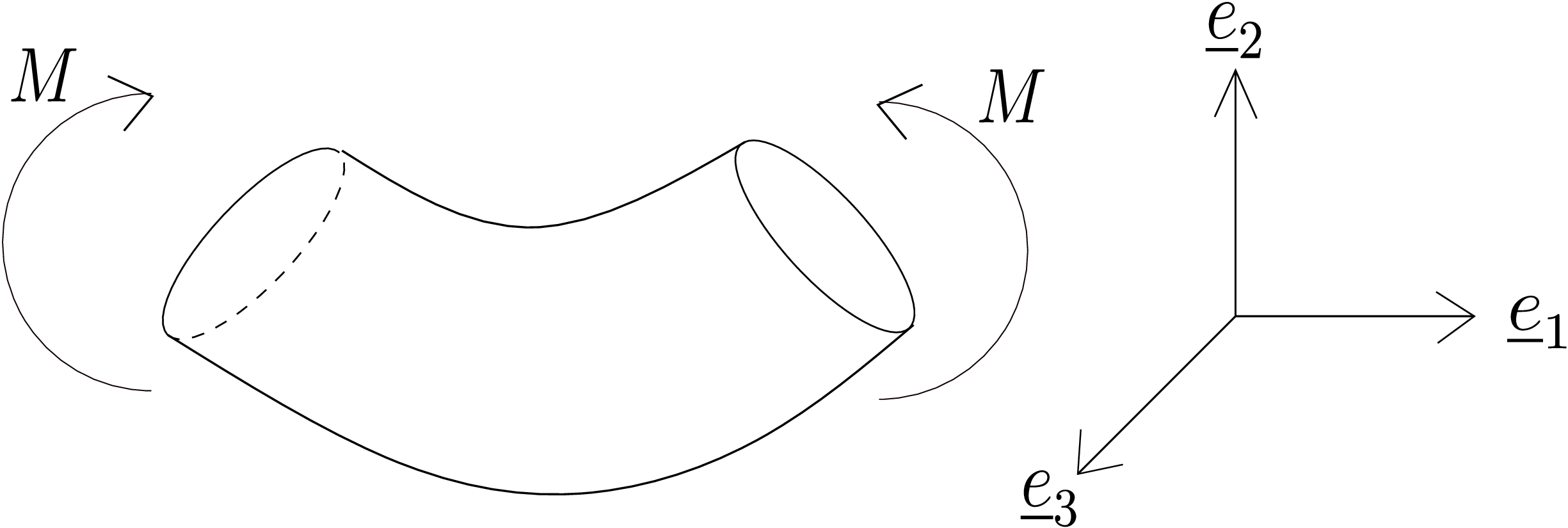
We can recall that the state of stress for such a case is given by \begin {equation} \begin {bmatrix}\underline {\underline {\sigma }}\end {bmatrix}= \begin {bmatrix} \sigma _{11} & 0 & 0\\ 0 & 0 & 0\\ 0 & 0 & 0 \end {bmatrix}. \end {equation} This is because the cross-section again relaxes freely in the transverse direction in case of pure bending. We had also derived that
Here \(\kappa \) denotes the bending curvature and \(y\) denotes distance from the neutral axis. Thus, the cross-sectional energy will be
The final integration over the cross-section yields
If we compare this form of bending energy with the extensional/stretching energy form \eqref{10_stretching_energy}, we can see that the form of both the energies is exactly the same: the axial force \(P\) is replaced by bending moment \(M\) while the stretching stiffness \(EA\) is replaced by bending stiffness \(EI_{zz}\).
In case of torsion, the state of stress in cylindrical coordinate system is \begin {equation} \begin {bmatrix}\underline {\underline {\sigma }}\end {bmatrix}= \begin {bmatrix} 0 & 0 & 0\\ 0 & 0 & \tau _{\theta z}\\ 0 & \tau _{\theta z} & 0 \end {bmatrix}. \end {equation} We had also derived earlier that
Here \(\kappa \) denotes twist, \(r\) denotes radial coordinate relative to the cross-section’s centroid and \(T\) denotes the internal torque or twisting moment. Thus, the cross-sectional energy will be
The final integration over the cross-section yields
We had learnt earlier that the presence of transverse load leads to non-uniform bending of beams which also generates transverse shear stress in beams - this shear stress points in the direction of applied transverse load and is different from the one due to torsion.§ Proceeding along the similar lines as earlier, the total shear energy due to transverse load turns out to be \begin {equation} E_{shearing}=\frac {V^2}{2k_sGA}. \end {equation} Here \(V\) represents shear force, \(GA\) shearing stiffness and \(k_s\) shear correction factor.
When we apply general load on a beam, force and moment both act on the cross-section (see Figure 10.10).
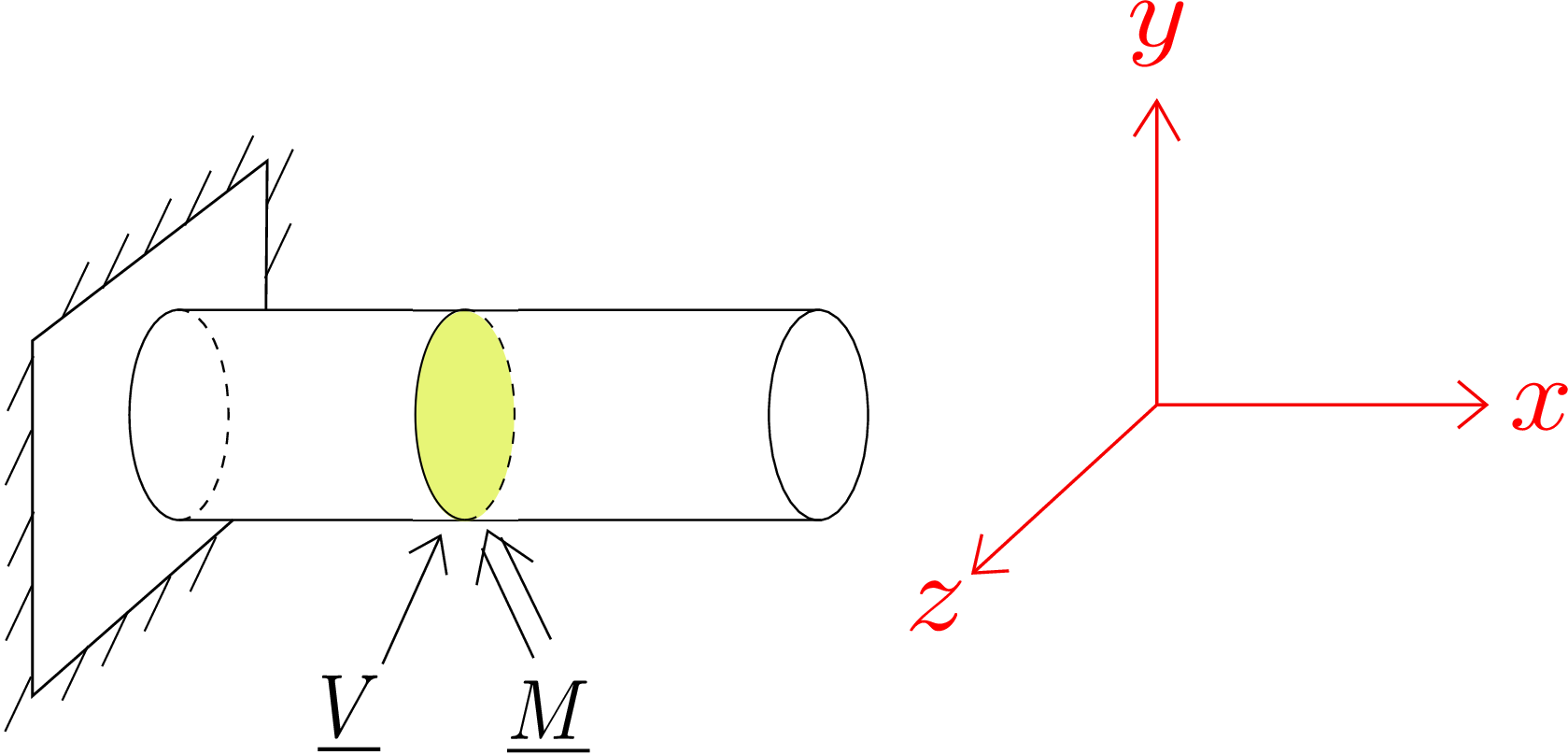
The internal force \(\underline {V}\) in the cross-section can be decomposed into three components as \begin {equation} \begin {bmatrix}\underline {V}\end {bmatrix}= \begin {bmatrix} V_x & V_y & V_z \end {bmatrix}^T. \end {equation} The component along the axis \(V_x\) is axial force \(P\). The other components are shear forces. We can similarly resolve the internal moment into three components as \begin {equation} \begin {bmatrix}\underline {M}\end {bmatrix}= \begin {bmatrix} M_x & M_y & M_z \end {bmatrix}^T. \end {equation} The component along the axis \(M_x\) is the torque \(T\). The other two components are bending moments. We derived energy due to each of these six components separately assuming only one of them was present. For the general case, can we sum individual energies? It turns out we cannot since individual energies are quadratic in applied generalized forces. However, if we resolve internal force and moment along principal directions, one can show that the total cross-sectional energy will indeed be simply the summation of energies of individual modes, i.e., \begin {equation} \label {10_final_energy} E=\int _0^L\Bigg [\frac {P(x)^2}{2EA}+\frac {M_y(x)^2}{2EI_{zz}}+\frac {M_z(x)^2}{2EI_{zz}}+\frac {T(x)^2}{2GJ}+\frac {V_y(x)^2}{2kGA}+\frac {V_z(x)^2}{2kGA}\Bigg ]dx. \end {equation} The first three terms here are due to normal strain whereas the last three terms are due to shear strain.
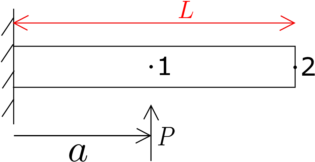
Solution: Let us first obtain the beam’s tip rotation, i.e., \(\theta (L)\). Let us solve it using Euler-Bernouli beam theory. We denote the point at which \(P\) is acting as point 1 and the free end as point 2. According to EBT: \begin {equation} \label {10_EBT} EI\frac {d^2y}{dx^2}=M(x). \end {equation} The bending moment profile can be found by cutting a section in the beam and analyzing one of its portions. It turns out to be
Here we are writing the force \(P\) as \(F_1\) since it is acting at point 1. Substituting this moment profile in equation \eqref{10_EBT} gives:
Integrating the expression for \(x<a\) twice gives \begin {equation} EIy=F_1a\frac {x^2}{2}-F_1\frac {x^3}{6}+C_1x+C_2. \end {equation} The boundary condition at the clamped end is
which when applied yields
Thus, we get \begin {equation} y=\frac {F_1}{EI}\bigg (a\frac {x^2}{2}-\frac {x^3}{6}\bigg ) \end {equation} and its derivative gives cross-sectional rotation \(\theta \), i.e., \begin {equation} \label {10_theta_right} \theta =\frac {dy}{dx}=\frac {F_1}{EI}\bigg (ax-\frac {x^2}{2}\bigg ). \end {equation} The above two relations hold for \(x\leq a\) only. In order to obtain expression for \(x>a\), we set \(M=0\) in EBT theory, i.e.,
Thus, \(\theta \) is constant in the segment from \(x=a\) to \(x=L\) which implies \begin {equation} \theta (L)=\theta (a)=\frac {F_1a^2}{2EI}. \end {equation} The second equality is obtained after enforcing continuity of rotation at \(x=a\) and further evaluating equation \eqref{10_theta_right} at \(x=a\). The above equation gives us influence coefficient relating \(\theta \) at point 2 with force at point \(1\), i.e., \begin {equation} \theta _2=\underbrace {\frac {a^2}{2EI}}_{k_{21}}F_1 \end {equation} We can also find \(k_{12}\) to check whether it comes out to be equal to \(k_{21}\). To obtain \(k_{12}\), we apply a bending moment \(M_2\) at point 2 and measure the deflection at point 1 (see Figure 10.11).
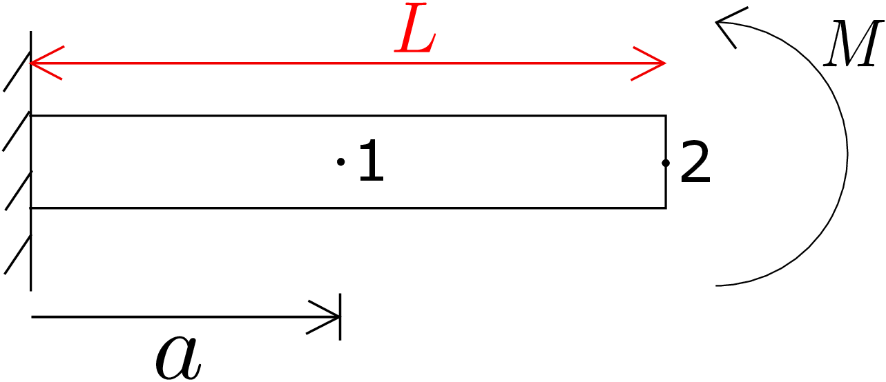
In this case, bending moment will be constant all along the length of the beam and equal to the applied moment \(M_2\). Substituting this in equation \eqref{10_EBT}, we get
The boundary conditions at the clamped end are the same as before (see \eqref{10_BC_EBT}), which again yield \(C_1=C_2=0\). Thus, we get \begin {equation} y=\frac {M_2~x^2}{2EI} \end {equation} using which the deflection at point 1 turns out to be \begin {equation} y_1=y(a)=\underbrace {\frac {a^2}{2EI}}_{k_{12}}M_2. \end {equation} We can see that \(k_{12}\) is the same as \(k_{21}\). Thus, we are able to verify the reciprocal relation. As we can see, the second problem of pure bending is much easier to solve than the first problem of finding the tip rotation. If we are asked to solve for tip rotation, we actually need \(k_{21}\). But if we can find \(k_{12}\) instead in a simple way (as we saw above), we can then use reciprocal relation to set it equal to \(k_{21}\). Thus, reciprocal relation turns out to be very useful in obtaining solution to a difficult problem by solving a simpler problem.
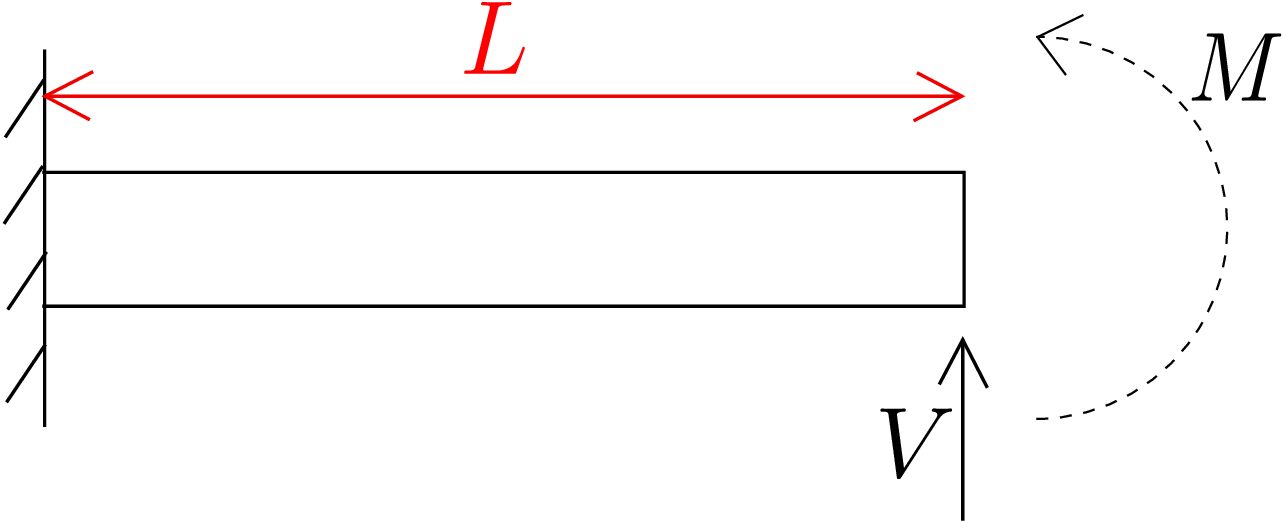
Solution: We want to find the rotation of the cross-section at the tip of the beam using energy method. The corresponding displacement of shear force is tip deflection. In order to find the rotation at the tip, a bending moment would also be needed to be applied at the tip: the unknown \(\theta (L)\) is the corresponding displacement of bending moment \(M(L)\). So, the steps needed to be followed are:
To obtain the beam’s energy, we first need shear force and bending moment profiles along the length of the beam. If we cut a section in the beam at a distance \(x\) from the clamped end and balance forces and moments in the right part of the cut beam, we will find that
The axial force \(P\), shear force \(V_z\), torque \(T\) and bending moment \(M_y\) are all zero here. Using these in equation \eqref{10_final_energy}, we get
We have thus been able to write the energy stored in the beam in terms of the externally applied loads (\(V\) and \(M\)). To obtain \(\theta _L\), we now apply Castigliano’s first theorem, i.e.,
As \(V\) and \(M\) are independent quantities, \(\frac {\partial V}{\partial M}\) would be zero which leads to \begin {equation} \theta _L=\int _0^L\frac {2(M+V(L-x))}{2EI_{zz}}dx \end {equation} We finally set \(M=0\) to obtain
For an exhaustive set of solved examples and unsolved objective and subjective type questions, please refer to the printed book.
∗If we consider large deformation problem, then stress-strain relation and strain-displacement relation become nonlinear.
†In the quasistatic process, the work done by the external agent exactly equals the energy stored in the spring since no part of the work done is dissipated.
‡Note that rotation is dimensionless
§In torsion of beams, total shear force due to shear stress \(\tau _{\theta z}\) is zero whereas the resultant shear force due to shear stress under transverse loading is obviously non-zero.