Having learnt about extension, torsion and bending of beams, we will now learn about two classical beam theories, i.e., Euler-Bernouli beam theory and Timoshenko beam theory which are used to obtain the beam’s transverse deflection when they are subjected to transverse load and couple. We will further discuss buckling of beams.
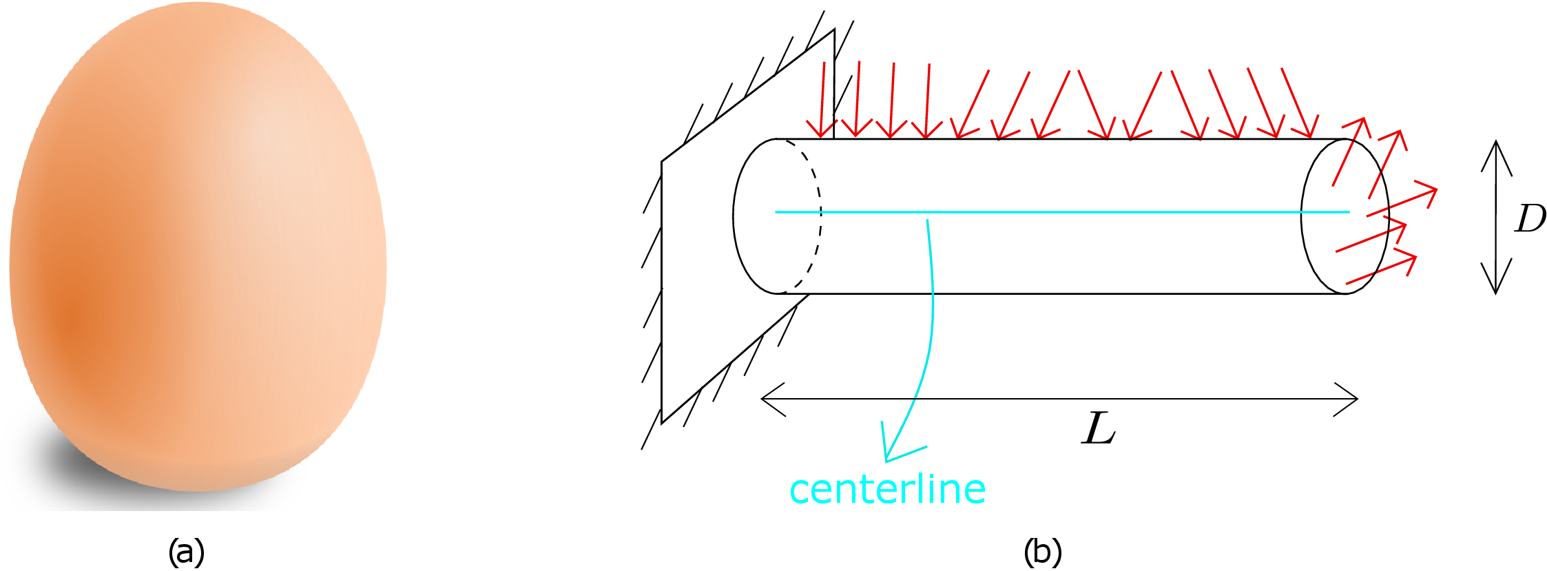
A beam is a slender body whose two of the dimensions are very small compared to its third dimension. It is geometrically characterized by its length and cross-section. A beam is also characterized by its aspect ratio or slenderness ratio which is defined as the ratio of its length to a representative size of the cross-section such as its diameter. The aspect ratio of a beam is usually of the order of 10 or higher. The body shown in Figure 9.1a is not a beam since it does not have a well-defined length or cross-section whereas the body shown in Figure 9.1b qualifies to be a beam. When applying load (e.g., terminal force/moment, distributed load etc. as shown in Figure 9.1b) to a beam, we want to know how it deflects.
The beam in Figure 9.1b has some general traction acting on its top and right surfaces. If we want to obtain its deformation, we can always use the following three-dimensional stress equilibrium equations:
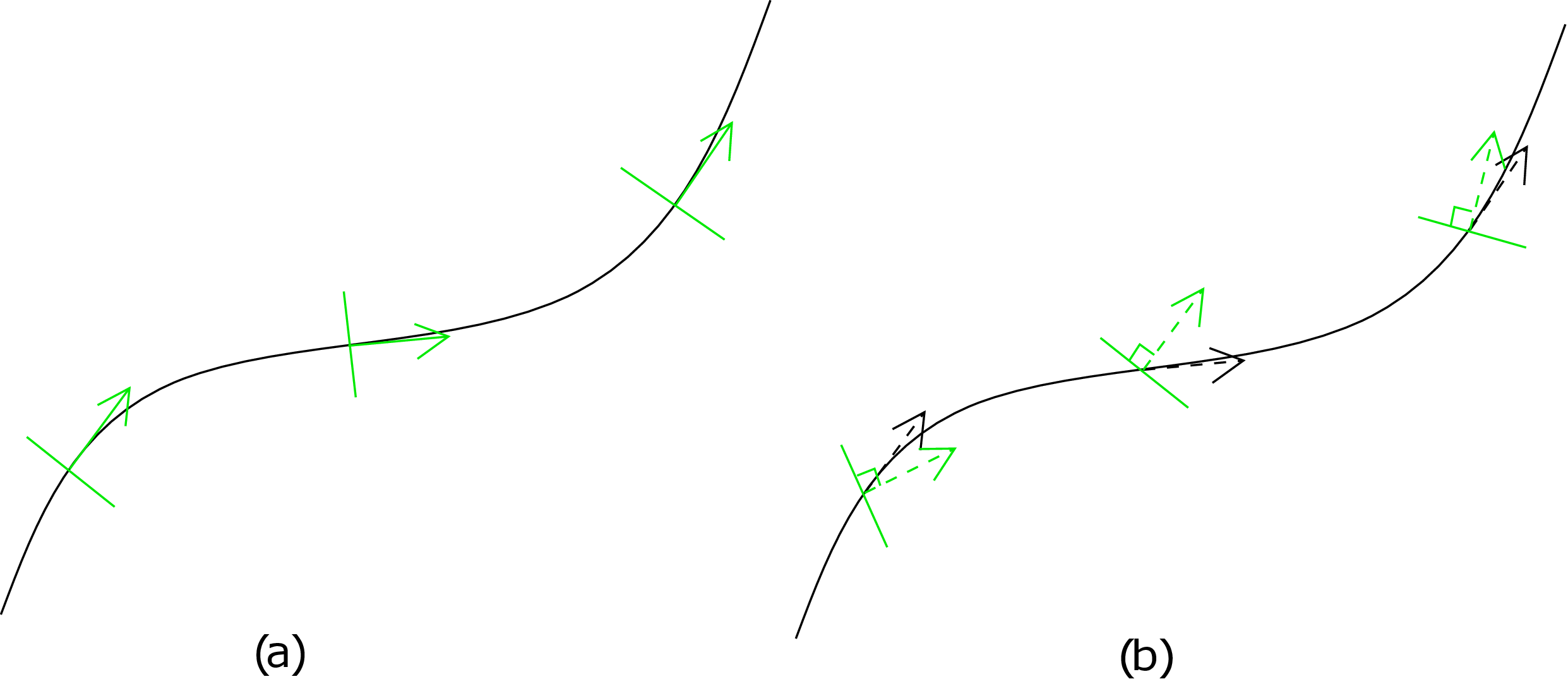
which is essentially a system of partial differential equations in three dimensions. We need to further plug in the stress-strain relation and the strain-displacement relations to finally obtain the equations in terms of the unknown displacement (\(\underline {u}(\underline {X})\)) of every point of the three-dimensional beam. It is usually impossible to solve such equations using pen and paper for an arbitrarily shaped body or even for a beam having arbitrary cross-section in which case we resort to numerical techniques. In beam theory, we look for an alternate and easier method to find the deformation of beams. The goal is not to find the displacement of every point of the beam but just its centerline which is typically the line joining the geometric centre of all its cross-sections. If we draw the exact deformed beam subjected to arbitrary loading, it might look as shown in Figure 9.2a: the displacement of every point of the beam is required to draw it.
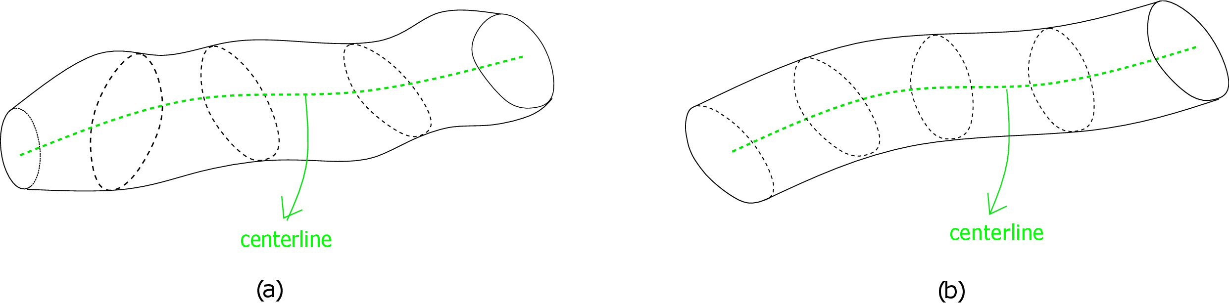
However, if we can accurately find just the deformed centerline and the deformed orientation of the beam’s
cross-section, we would get an approximate deformed beam as shown in Figure 9.2b. Here all the
cross-sections are kept rigid and just drawn about the deformed centerline: the envelope of these
cross-sections forms the approximate deformed beam. It turns out that if the beam is slender enough (i.e.,
the aspect ratio is greater than 10), the cross-section deformation is indeed negligible and the approximate
deformed beam shown in Figure 9.2b is then a an excellent approximation of the actual deformed beam.
Thus, for deformation problems involving slender beams, we can just solve for its centerline and place the
cross-sections rigidly about the centerline to construct the entire three-dimensional deformed beam. This is
the essence of beam theory.
Let us consider the placement of rigid cross-sections more closely. Once we have obtained the deformed
centerline, there are various ways to place the rigid cross-sections on it. The cross-section can be placed
such that its plane normal is oriented arbitrarily as shown in Figure 9.3a or one can
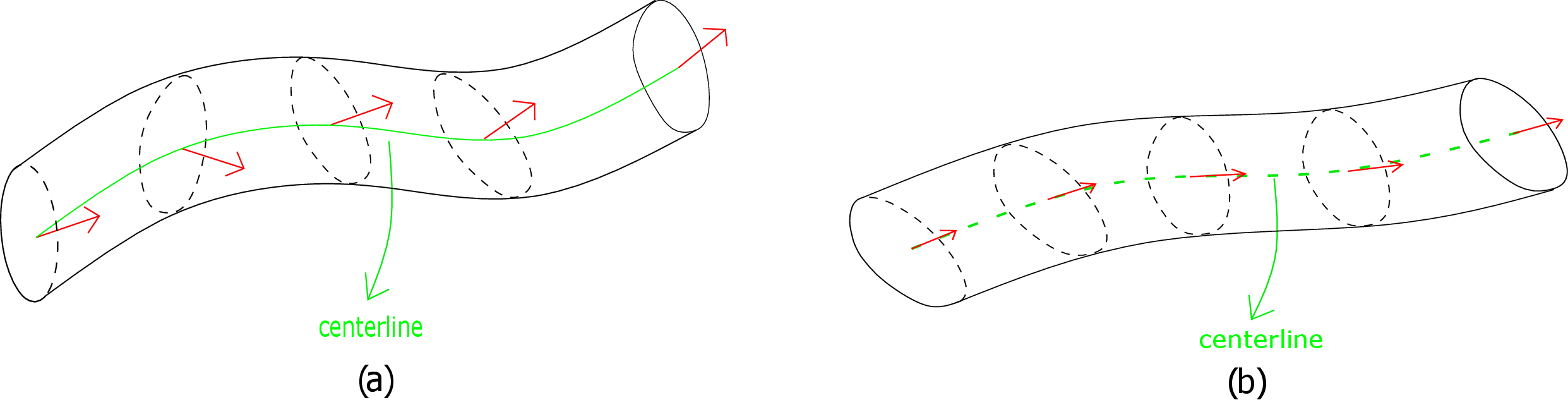
align the cross-section normal with the deformed centerline tangent as in Figure 9.3b. Thus, a beam theory, in general, solves for both the beam’s centerline and cross-section orientation. It turns out that the equations required to get these two variables are simple ordinary differential equations which are much easier to solve than the three-dimensional partial differential equations in \eqref{9_pde}. In fact, it would also be possible to obtain analytical solution to the ODEs of beam theory in many cases.
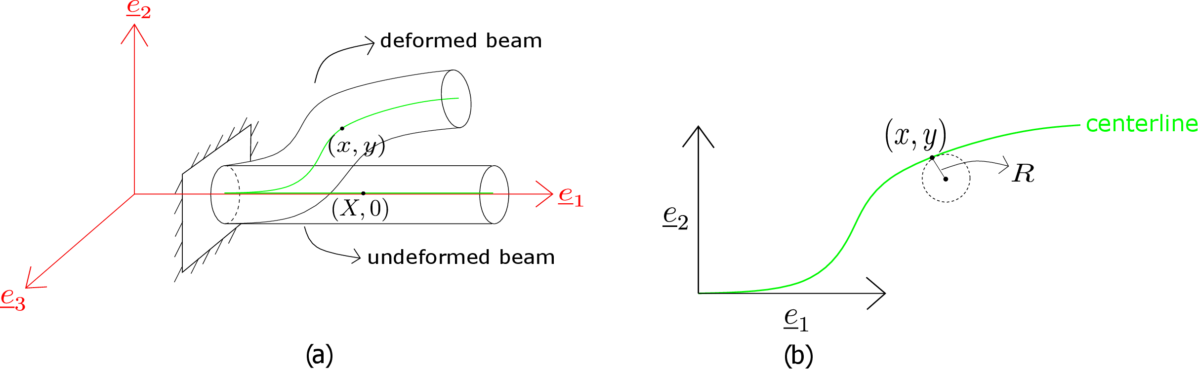
In this theory, it is assumed that the centerline tangent and the cross-section normal are aligned (see Figure 9.3b). Thus, the centerline is the only unknown. To get the required equation for it, we use the following bending formula derived earlier: \begin {equation} \label {9_bending_equation} M=EI\kappa . \end {equation} Here \(M\) represents bending moment, \(EI\) bending stiffness and \(\kappa \) bending curvature. We also know from differential geometry that the curvature \(\kappa \) of a curve can be written as \begin {equation} \label {9_differential_geometry} \kappa =\frac {\frac {d^2y}{dx^2}}{\big (1+\big (\frac {dy}{dx}\big )^2\big )^\frac {3}{2}} = \frac {M}{EI} \end {equation} where \((x,y)\) denotes the coordinates of a point on the curve. We can apply the above formula to the beam’s centerline with \(y\) denoting its transverse deflection (see Figure 9.4a) from the initial straight configuration.∗† The above equation is nonlinear in the unknown deflection \(y\).
The horizontal coordinate \(x\) is also an unknown. In the Euler-Bernouli beam theory, the axial displacement is assumed to be negligible. This means that the deformed axial coordinate \(x\) and the undeformed axial coordinate \(X\) are approximately the same, i.e., \begin {equation} x\approx X. \end {equation} Accordingly, the curvature formula can be approximated by \begin {equation} \label {9_kappa_x} \kappa \approx \frac {\frac {d^2y}{dX^2}}{\big (1+\big (\frac {dy}{dX}\big )^2\big )^\frac {3}{2}}. \end {equation} To linearize the above expression in deflection \(y\), it is further assumed that the magnitude of the slope of the centerline is very small, i.e., \begin {equation} \bigg |\frac {dy}{dX}\bigg |\ll 1 \end {equation} using which equation \eqref{9_kappa_x} becomes \begin {equation} \kappa (X)\approx \frac {d^2y}{dX^2}. \end {equation} The curvature now becomes linear in transverse deflection. Substituting the above relation in equation \eqref{9_bending_equation}, we get \begin {equation} \label {9_EBT} \boxed {EI\frac {d^2y}{dX^2}=M(X)} \end {equation} which is the governing equation of the Euler-Bernouli beam theory (EBT). To summarize, the following assumptions are made in deriving the equations of Euler-Bernouli beam theory:
Let us solve some beam deflection problems using this beam theory.
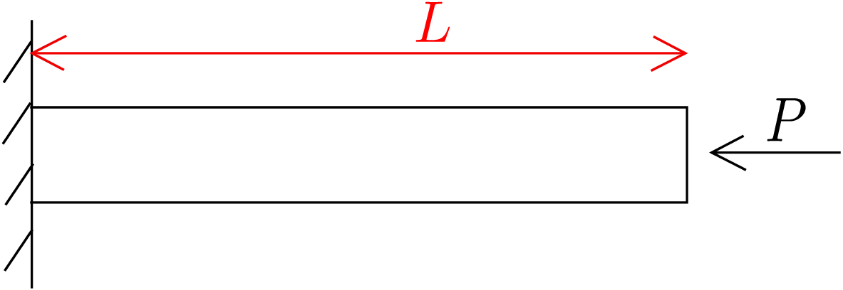
Suppose we have a straight beam which is clamped at one end and is subjected to a transverse load \(P\) at its other end as shown in Figure 9.5.
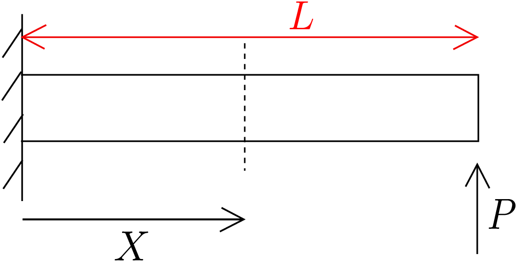
Let us obtain the deflection of this beam using the Euler-Bernouli Theory (EBT). We first need to find the bending moment profile (i.e., bending moment M as a function of \(X\)). Let us cut a section in the beam at a distance \(X\) from the clamped end. The free body diagram of the resulting two parts of the beam are shown in Figure 9.6.
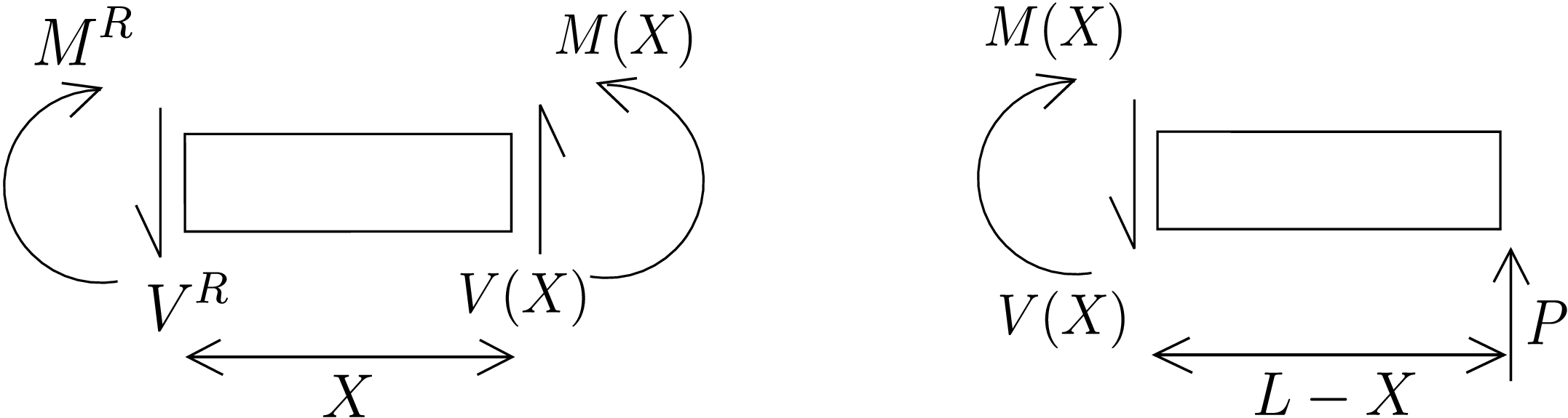
For the left part of the beam, at its right end, the cross-section normal points in \(+x\) direction. Therefore, here the shear force V(X) will act upward and the bending moment M(X) will act in anticlockwise direction. The reactive shear force and reactive bending moment from the clamped support are also shown at the left end of this part. If we consider the right part of the beam, external force \(P\) acts at its rightmost end. As the cross-section normal of its left end points in \(-x\) direction, the shear force V(X) acts on it in \(-y\) direction. Similarly, the bending moment M(X) at the left end acts in clockwise direction as per convention. Moment balance for the right part of the beam about the centroid of its left-end cross-section results in
Plugging this expression in equation \eqref{9_EBT}, we get \begin {equation} \label {9_example1_equation} \frac {d^2y}{dX^2}=\frac {P}{EI}(L-X). \end {equation} This is a second order linear differential equation. So, we need two boundary conditions to solve it. If there were additional unknown parameter in the equation, we would have required more boundary conditions to find them. At the clamped end (\(X=0\)), the centerline cannot deflect and the cross-section cannot rotate either. As the cross-section normal has to be aligned with the centerline tangent in this theory, the slope of the centerline itself will give us the cross-section normal. Thus, we get the following two boundary conditions:
Integrating equation \eqref{9_example1_equation}, we obtain \begin {equation} \frac {dy}{dX}=\frac {P}{EI}\bigg (LX-\frac {X^2}{2}\bigg )+C_1 \end {equation} The constant \(C_1\) turns out to be zero upon applying the boundary condition \eqref{9_BC2}. Integrating further, we get \begin {equation} y=\frac {P}{EI}\bigg (L\frac {X^2}{2}-\frac {X^3}{6}\bigg )+C_2 \end {equation} The constant \(C_2\) also turn out to be zero upon using the other boundary condition, i.e., equation \eqref{9_BC1}. Thus, we get
The tip deflection can be obtain by substituting \(X=L\) in the above equation which yields \begin {equation} y^{tip}=y(L)=\frac {PL^3}{3EI}. \end {equation} Thus, larger the force, larger is the tip deflection. Also, larger the bending stiffness \(EI\), smaller is the deflection.
In this example, we think of a simply supported beam as shown in Figure 9.7. Unlike clamped supports, simple supports do not exert reactive bending moment on the beam. They consist of line contacts. If we have a line contact between the beam and the support, the contact traction will obviously pass through the contact line as shown in Figure 9.7.
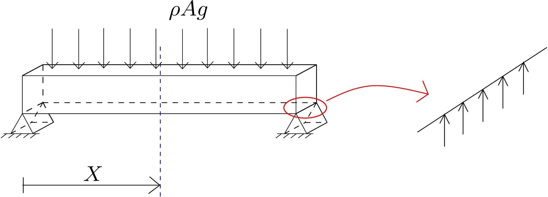
So, the moment due to this line force about the contact line itself will always be zero.‡ As the line contacts at the support are along \(z\) axis, there is no reactive moment at the two ends about \(z\) axis. The beam is also subjected to a constant distributed load. To visualize this distributed load, we can also think of it as the weight of the beam itself in which case the distributed load will be equal to \(\rho gA\) where \(\rho \) and \(A\) denote the beam’s density and cross-sectional area, respectively. Although, the reactive bending moment at the two ends is zero, the reactive transverse load is present. This is because the beam is restricted by the support and cannot move downwards. This reactive transverse load will be equal to the integration of the traction over the line contact (see the zoomed view of line contact in Figure 9.7). As a rule of thumb, one can remember the following table while applying boundary condition for different types of support:
| Transverse displacement | Transverse Load |
| 0\(~\Rightarrow \) | \(\times \) |
| \(\times \) | \(\Leftarrow ~0\) |
| Rotation(\(z\)) | Moment(\(z\)) |
| 0 \(~\Rightarrow \) | \(\times \) |
| \(\times \) | \(\Leftarrow ~\) 0 |
Here ‘\(\times \)’ implies that the corresponding quantity is an unknown and may be non-zero. For example, if the applied transverse load at an end is zero, then the displacement at that end in the direction of the loading is an unknown. If the applied moment at an end is zero, then the rotation at that end is an unknown. For our beam (shown in Figure 9.7), the displacement of the beam in \(y\) direction is restricted at the ends. So, the transverse load in the same direction is an unknown. Also, the bending moment about \(z\) axis is zero at the ends which implies the end-rotation about \(z\) axis is an unknown.§ To obtain deflection, we have to solve equation \eqref{9_EBT} for which we again require the bending moment profile. So, we cut a section at a distance \(X\) from the left end of the beam and draw the free body diagram of the right part of the beam as shown in Figure 9.8.
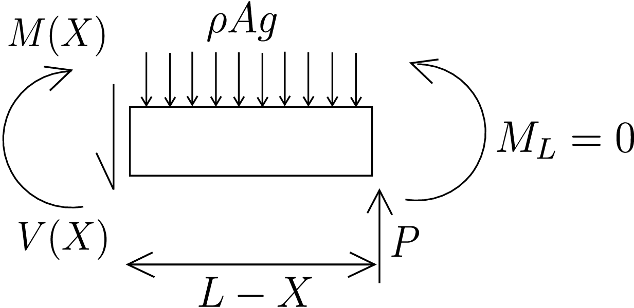
On its left-end cross-section, shear force \(V(X)\) is directed downwards while the bending moment \(M(X)\) is clockwise. On the right-end cross-section, bending moment is zero while some unknown shear force \(P\) acts in the upward direction. Moment balance about the centroid of the left-end cross-section is now carried out. The contribution due to the distributed load is calculated by replacing the distributed load by a single equivalent force acting at the center of this part of the beam. Thus, we finally get
We can now substitute this expression of \(M(X)\) in equation \eqref{9_EBT} to get \begin {equation} \label {9_before_P} \frac {d^2y}{dX^2}=\frac {P}{EI}(L-X)-\frac {\rho Ag}{EI}\frac {(L-X)^2}{2}. \end {equation} As pointed earlier, we require one extra boundary condition (total 3) due to the presence of the unknown parameter \(P\). The three boundary conditions are vanishing of transverse displacement at the two ends and vanishing of bending moment at the left end: we have already used vanishing of bending moment at right end in deriving \eqref{9_example2_moment}. Upon setting \(M(0)=0\) in equation \eqref{9_example2_moment}, we get \begin {equation} P=\frac {\rho AgL}{2}. \end {equation} This means that the reactive transverse load by the support is equal to half of the total load due to distributed force. Substituting the above expression of \(P\) in equation \eqref{9_before_P}, we get
Upon further integrating it twice, we obtain
Finally, we use the following two remaining boundary conditions:
to obtain \((C_1,C_2)\) which yields
The maximum deflection turns out to be at the mid point of the beam where the slope of the centerline vanishes.
In Euler-Bernouli beam theory, it was assumed that the centerline tangent and the cross-section normal are aligned as shown in Figure 9.9a.
So, we have only one kinematic variable which is the deflection of the beam \(y\): we can obtain the cross-section orientation from its derivative, i.e., \(\frac {dy}{dX}\). However, in Timoshenko Beam Theory (TBT), we do not assume the centerline tangent and cross-section normal to be aligned as shown in Figure 9.9b. Thus, this is a more general theory than EBT: we have deflection \(y\) and cross-section rotation \(\theta \) as two independent unknowns here. We will now derive the governing equations of this new theory. Let us consider a beam which is initially straight as shown in Figure 9.10a and gets deformed due to some arbitrary loading.
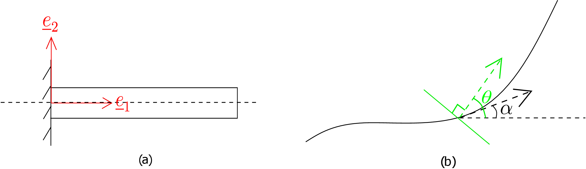
Let us focus on a typical cross-section of the beam in its deformed configuration as shown in Figure 9.10b. The centerline tangent makes an angle \(\alpha \) with the horizontal which implies
The deformed cross-section normal makes an angle \(\theta \) with the horizontal. Thus, the angle between the cross-sectional line (shown as solid green line in Figure 9.10b: it should not be confused with cross-section normal) and the centerline tangent becomes
In the undeformed straight beam, this angle between the cross-sectional line (which lied along \(\textbf {e}_2\) axis originally) and the centerline tangent (which lied along \(\textbf {e}_1\) axis originally) was \(\frac {\pi }{2}\). As shear strain measures the changes in angle (initial-final) between initially perpendicular line elements, we have
The superscript \((^0)\) here denotes the fact that it is the shear strain at the centroid of the cross-section since one of the perpendicular lines, i.e., the beam centerline passes through the centroid of the cross-section. Let us relate this centroidal shear strain to the total shear force acting in the cross-section. Suppose \(V\) represents the shear force acting in the cross-section and \(A\) the cross-sectional area. The average shear stress \(\tau _{xy}\) in the cross-section will then be \begin {equation} \tau _{xy}^{avg}=\frac {V}{A}. \end {equation} If we further assume rectangular cross-section for the beam, we had seen earlier that the value of shear stress at the centroidal line is \(\frac {3}{2}\tau ^{avg}\), i.e.,
The factor \(\frac {2}{3}\) is the shear correction factor \(k^s\) for rectangular beams which is different for different cross-section shapes. Further, using linearly isotropic stress-stress relationship, we get
Substituting this in equation \eqref{9_gamma_geometric}, we finally get \begin {equation} \label {9_TBT1} \boxed {\frac {dy}{dX}-\theta =\frac {V}{k^sGA}} \end {equation} This is one of the equations of TBT. It accounts for the effect of shear force which is neglected in EBT. We need one more equation which comes from moment-curvature relation, i.e., \begin {equation} \label {9_bending_equation_1} EI~\kappa =M. \end {equation} In EBT, we could write the bending curvature as the curvature of the centerline. But in TBT, bending curvature is no more equal to the curvature of the centerline since the centerline is also undergoing shear.¶ Accordingly \begin {equation} \kappa \neq \frac {d^2y}{dX^2}. \end {equation} In TBT, we can relate the bending curvature to cross-section rotation \(\theta \). Figure 9.11 shows a beam bent into an arc of a circle of radius \(R\).
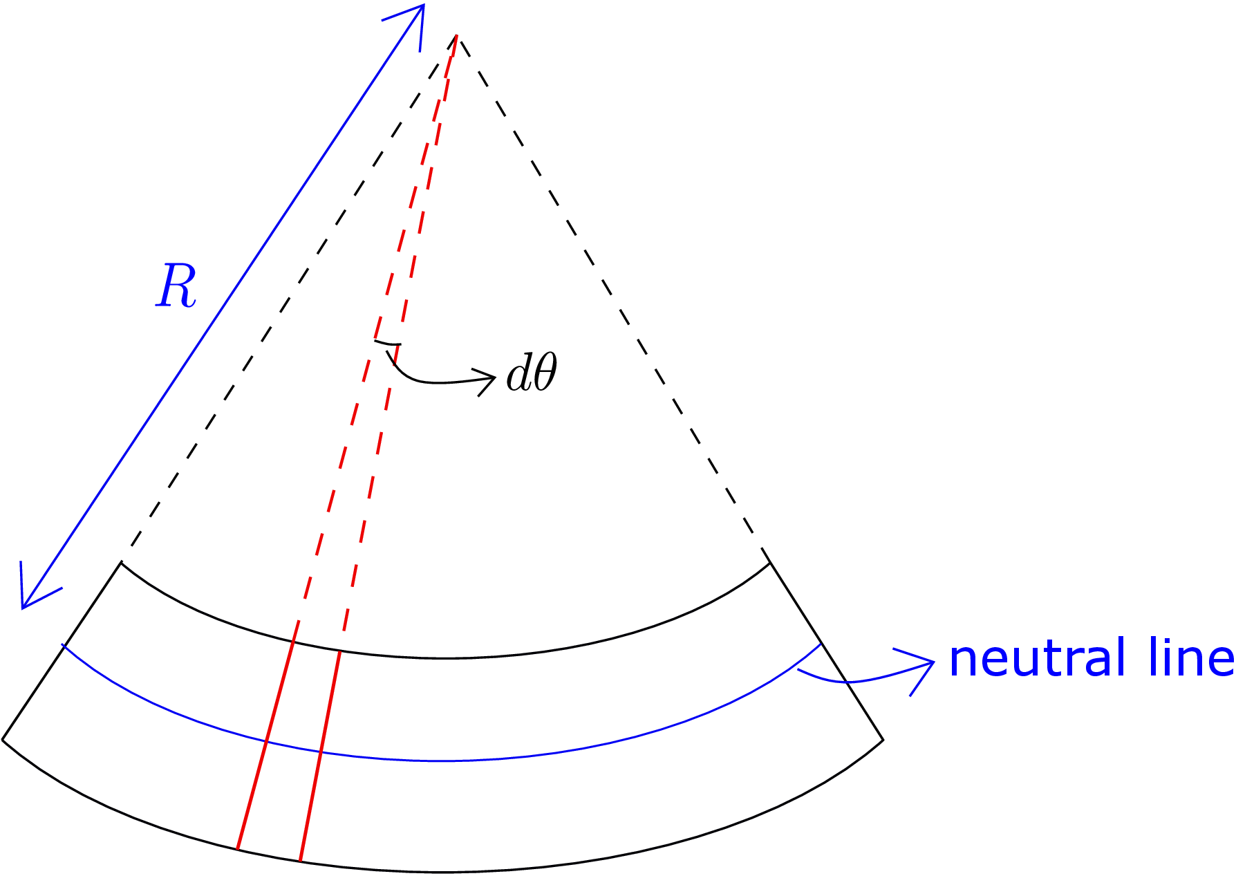
Let us focus on two cross-sections located very close to each other (shown by solid red lines in the Figure). The relative rotation between the two cross-sections is the same as the angle subtended by the arc joining the two cross-sections at the center (shown by \(d\theta \)). As the neutral axis does not undergo any stretching, we can write
In fact, the above relation for bending curvature holds for both EBT and TBT. Plugging the above form for bending curvature into equation \eqref{9_bending_equation_1}, we get \begin {equation} \label {9_TBT2} \boxed {EI\frac {d\theta }{dX}=M(X)} \end {equation} This is a more general equation than the one used in Euler-Bernouli beam theory. We can compare the two theories as follows:
We have thus obtained the two equations for TBT (equations \eqref{9_TBT1} and \eqref{9_TBT2}) which form a system of coupled first order linear differential equations. Two boundary conditions will be needed to solve this system. In fact, more boundary conditions will be needed if shear force \(V(x)\) and bending moment \(M(x)\) contain unknown parameters.
Consider the problem that we had solved using EBT - see Figure 9.5. A transverse force \(P\) is applied at the free end of a beam which is clamped at the other one end. We would like to solve for the beam’s deflection using TBT and further compare the result with that of EBT. The first step is finding the shear force and bending moment profile in the beam. For that, as earlier we cut a section in the beam at a distance \(X\) from the clamped end and draw the free body diagram of the right portion of the beam as shown in Figure 9.6b. As earlier, moment balance about the centroid of the left end yields
whereas force balance yields \begin {equation} V(X)=P. \end {equation} Plugging them into equations of TBT (equations \eqref{9_TBT1} and \eqref{9_TBT2}), we get
We have two boundary conditions both at the clamped end. The displacement \(y\) and the cross-section rotation \(\theta \) must be zero here, i.e.,
We should keep in mind that we cannot set \(\frac {dy}{dX}=0\) as \(\frac {dy}{dX}\) no longer denotes rotation of the cross-section. Integrating equation \eqref{9_example_eq1}, we get \begin {equation} \theta =\frac {P}{EI}\bigg (LX-\frac {X^2}{2}\bigg )+C_1 \end {equation} Using equation \eqref{9_BC2_1} in it, we get \(C_1=0\). Now, we can plug the above expression for \(\theta \) in equation \eqref{9_example_eq2} to get \begin {equation} \frac {dy}{dX}=\frac {P}{EI}\bigg (LX-\frac {X^2}{2}\bigg )+\frac {P}{k^sGA} \end {equation} whose integration yields
This is the final expression for deflection \(y\) obtained by TBT. We get an extra term \(\frac {PX}{kGA}\) when we compare the result with the one from EBT.
Let us now explore which of the two theories to use in a given scenario. If the result from TBT is very close to the one from EBT, then we can simply apply EBT and neglect the effect of shear. The tip deflection from TBT can be found by substituting \(X=L\) in equation \eqref{9_cantilever_TBT} which yields \begin {equation} y^{L,TBT}=\frac {PL^3}{3EI}+\frac {PL}{k^sGA} \end {equation} whereas the tip deflection from EBT was \begin {equation} y^{L,EBT}=\frac {PL^3}{3EI}. \end {equation} Assuming the result from TBT to be more accurate, the relative error in EBT solution (\(\epsilon _r^{EBT}\)) will be
We can write the moment of area \(I_{zz}\) in terms of the cross-sectional area and radius of gyration of the cross-section (\(R_G\)). The radius of gyration \(R_G\) also depends on the shape and size of the cross-section. For a rectangular cross-section of height \(h\) and width \(b\), e.g.,
Plugging this into equation \eqref{9_before_Izz}, we get
For EBT to be applicable, the relative error must be very small, i.e.,
Here we have separated the geometric and material parameters: the geometric term on the left is the aspect ratio of the beam whereas the material parameter \(\nu \) on the right is the material’s Poisson’s ratio. For illustration, consider a case where the Poisson’s ratio \(\nu \) is 0.3 and the cross-section of the beam is rectangular. Thus, \(k^s=\frac {2}{3}\). Putting these values into the RHS of the above relation, we get \begin {equation} \frac {L^2}{R_G^2}\gg {\frac {6 \times 1.3}{\frac {2}{3}}}\approx 12. \end {equation} So, if the ratio \(\frac {L^2}{R_G^2}\) is much greater than 12 (e.g., 100), then we can use Euler-Bernouli Beam theory safely. For shorter beams having low aspect ratio, one would have to use Timoshenko beam theory.
When we try to compress a stick of a broom (or any long and thin rod), it initially remains straight as shown in Figure 9.12 but as we keep increasing the compressive force, it suddenly bends.
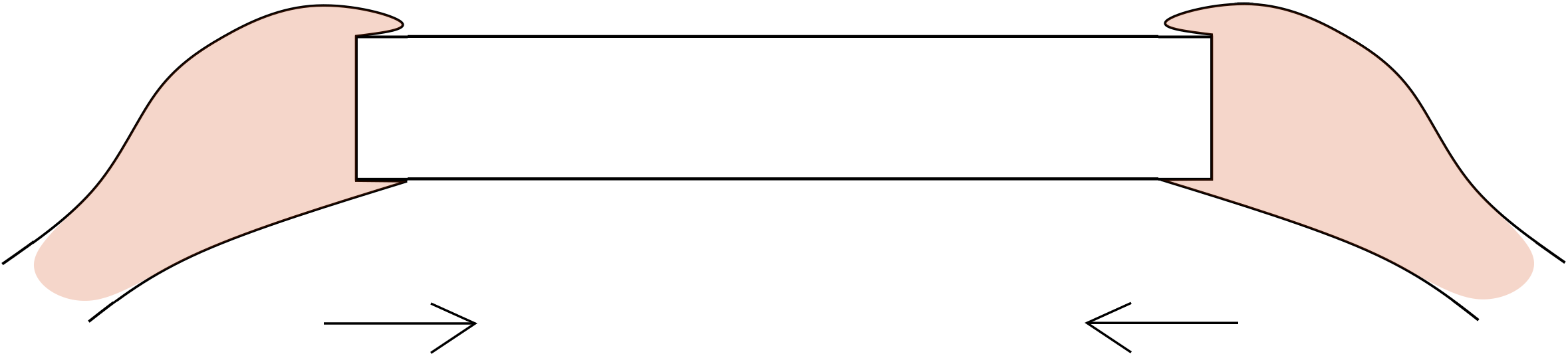
This is called buckling and the critical value of compressive load at which it bends is called the buckling
load. Whenever we design a machine having beam-like elements where it has to hold compressive load, we
have to make sure that the operative compressive load is less than the buckling load. Otherwise, the beam
element will buckle leading to the machine’s failure.
Let us now see how to obtain the buckling load. We will use EBT to model the beam. This means we are
neglecting the effect of shear which, as derived earlier, is a good assumption for long beams (aspect ratio \(>\)
10). We will consider the case of column buckling. i.e., a beam clamped at one end and subjected to an
axial compressive force at the other end (see Figure 9.13).
When the compressive load \(P\) reaches the critical value, the beam/column will bend as shown in Figure 9.14a even though we are applying axial compressive load here.
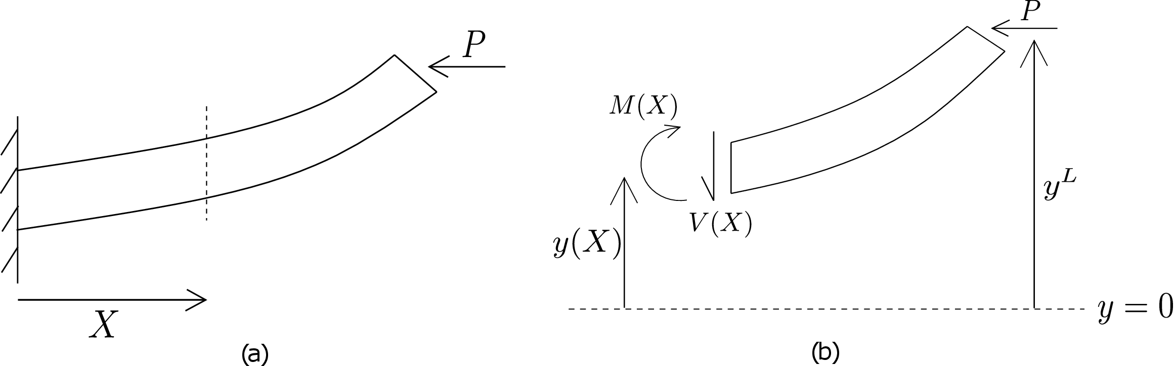
We want to find this critical load. Let us rewrite the equations of EBT: \begin {equation} \label {9_EBT_1} EI\frac {d^2y}{dX^2}=M(X). \end {equation} We need to first find the bending moment profile. For this, we cut a section in the beam at a distance \(X\) from the clamped end (see Figure 9.14a) and draw free body diagram of the right portion of the beam as shown in Figure 9.14b. The applied load \(P\) acts on its right-end while shear force \(V(X)\) and bending moment \(M(X)\) acts on its left end. The \(y\)-coordinate of the left and right ends are \(y(X)\) and \(y^L\), respectively. Moment balance about the centroid of the left-end cross-section yields
Upon substitute this in equation \eqref{9_EBT_1}, we get \begin {equation} \label {9_buckling_main} EI\frac {d^2y}{dX^2}+Py=Py^L. \end {equation} This is a second order non-homogeneous ordinary differential equation. To find its general solution, we need to first solve the corresponding homogeneous equation and then add particular integral to it. The corresponding homogeneous equation is \begin {equation} EI\frac {d^2y}{dX^2}+Py=0. \end {equation} We can note that \(P\) is positive as it is always compressive in nature. If \(P\) were a tensile load, it would become negative. Let us substitute \(y=e^{\lambda X}\) in the above equation which leads to the following characteristic equation:
Here \(i\) denotes the imaginary number \(\sqrt {-1}\). As \(\lambda \) is imaginary, the solution has cosine and sine terms. The complementary function can thus be written as \begin {equation} y=C_1\cos \bigg (\sqrt {\frac {P}{EI}}X\bigg )+C_2\sin \bigg (\sqrt {\frac {P}{EI}}X\bigg ). \end {equation} We can get the particular integral just by observation in this case. When we substitute \(y=y^L\) in equation \eqref{9_buckling_main}, we see that it satisfies the equation. As any solution/function that satisfies the differential equation can be considered as a particular integral, we therefore choose \(y=y^L\) as the particular integral. Thus, the general solution becomes \begin {equation} \label {9_buckling_solution_with_constants} y=C_1\cos \bigg (\sqrt {\frac {P}{EI}}X\bigg )+C_2\sin \bigg (\sqrt {\frac {P}{EI}}X\bigg )+y^L. \end {equation} To find the unknown constants \(C_1\) and \(C_2\), we need to use boundary conditions. At the clamped end, both deflection and cross-section rotation are zero, i.e.,
Differentiating equation \eqref{9_buckling_solution_with_constants}, we get \begin {equation} y'=-C_1\sin \bigg (\sqrt {\frac {P}{EI}}X\bigg )+C_2\cos \bigg (\sqrt {\frac {P}{EI}}X\bigg ). \end {equation} Substituting \(X=0\) in this equation, we get
Similarly, substituting \(X=0\) in equation \eqref{9_buckling_solution_with_constants}, we get
Thus, the solution becomes \begin {equation} y(X)=y^L\bigg (1-\cos \bigg (\sqrt {\frac {P}{EI}}X\bigg )\bigg ). \end {equation} To obtain \(P\), we can use the fact that the above expression must be equal to \(y^L\) if we substitute \(X=L\) in it, i.e.,
This is the expression for the buckling load. We can get multiple buckling loads by setting n=0,1,2,3 and so on. The smallest buckling load will be obtained for \(n=0\) which is the critical load that we had set out to obtain. Thus \begin {equation} P^{cr}=\frac {\pi ^2EI}{4L^2}. \end {equation} If the compressive force is greater than the above critical value, the beam will bend (buckle), otherwise it will simply remain straight. This critical load is proportional to bending stiffness \(EI\) and inversely proportional to square of the beam’s length. So, a longer beam requires lesser force to buckle than a shorter beam. This can also be experienced in day-to-day life. The above buckling solution was obtained by substituting the boundary conditions in the general solution \eqref{9_buckling_solution_with_constants}. If we apply different set of boundary conditions, we would obtain different expression for buckling load. For example, for a beam clamped at both the ends as shown in Figure 9.15,
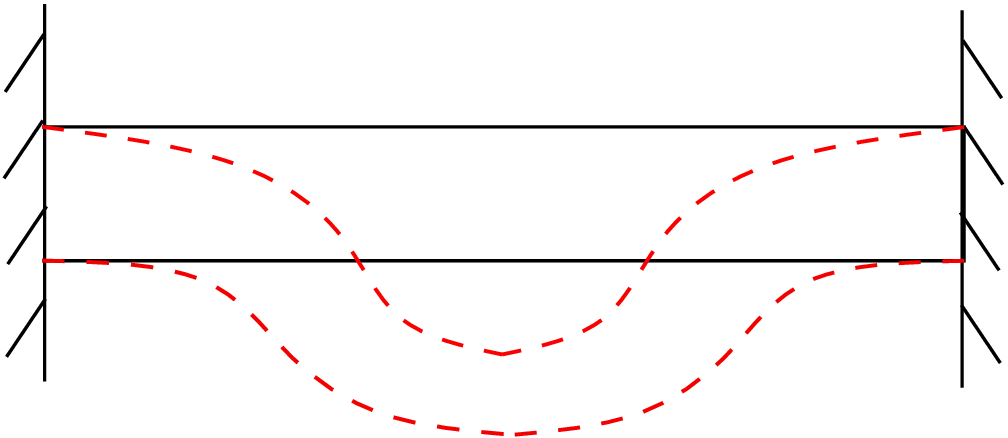
the buckling load turns out to be \begin {equation} P^{cr}=\frac {4\pi ^2EI}{L^2}. \end {equation} In fact, the buckled shape of the beam is also different (see the red dashed buckled solution in Figure 9.15). However, the buckling load is again inversely proportional to square of the beam’s length. With this, we close our discussion on beam theory.
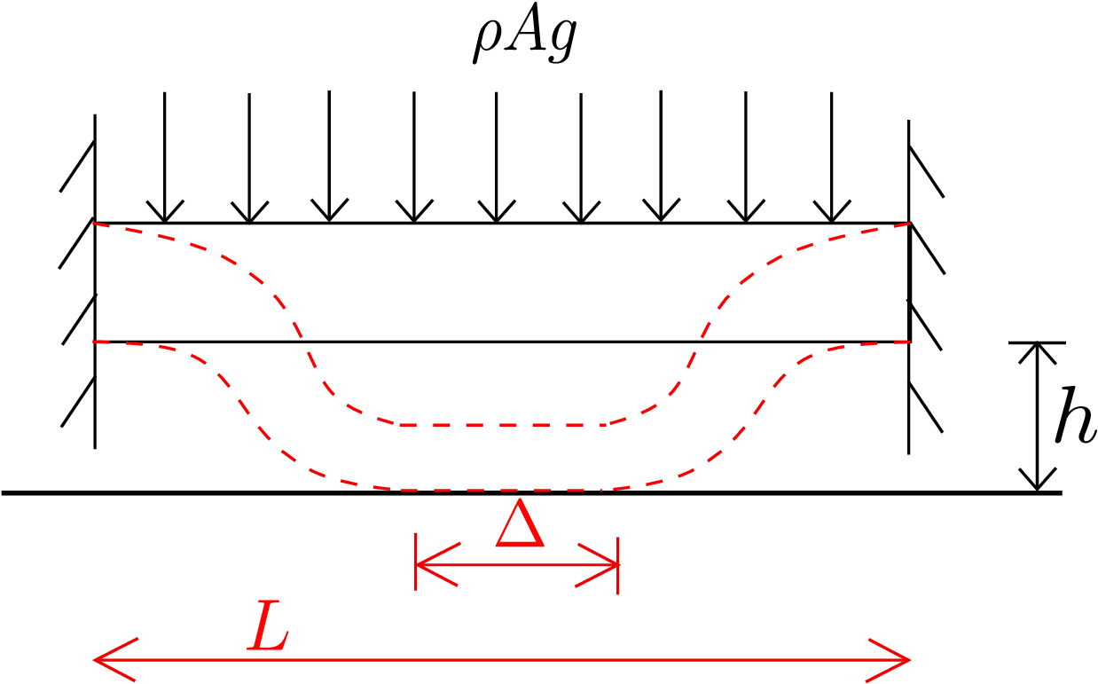
One can take the distributed load to be \(\rho Ag\). The ground position (\(h\) below the beam) is such that some part of the beam rests on the ground upon deformation while the remaining part just hangs. Find the portion of the beam \(\Delta \) which will rest on the ground. Use Euler-Bernouli beam theory. (NPTEL link)
Solution: First of all, we can notice that the problem is symmetrical with respect to the center of the beam (\(X=\frac {L}{2}\)). Let us consider the left hanging part of the beam, i.e., from \(X=0\) to \(X=\frac {L-\Delta }{2}\). We draw its free body diagram as shown in Figure 9.16a.
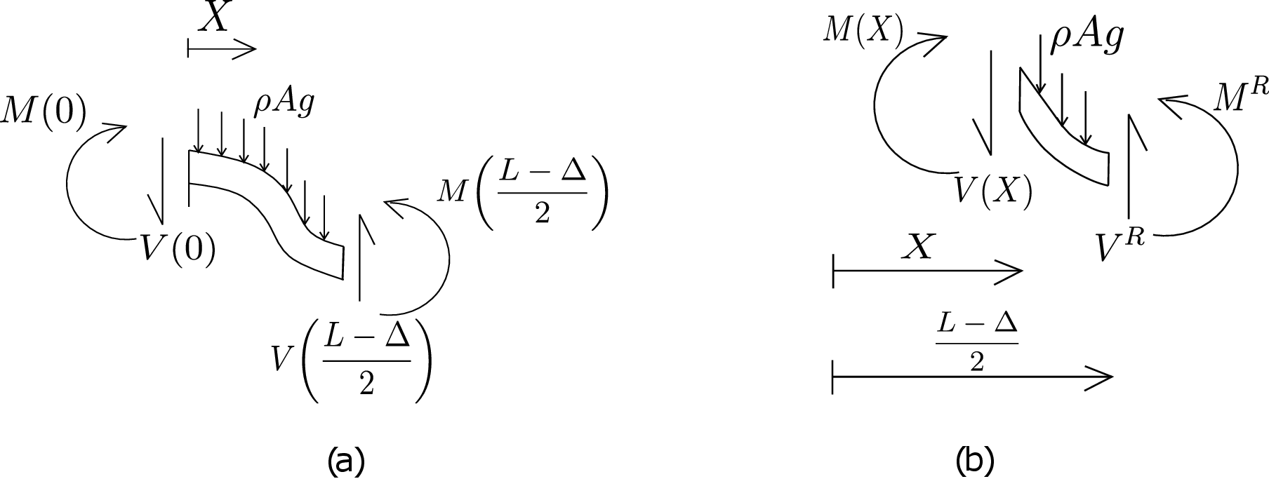
Bending moment \(M(0)\) and shear force \(V(0)\) act on its left-end cross-section (applied by the clamped end). A shear force and a bending moment also acts on the right-end of this part (applied by the remaining part of the beam). All of these four quantities are unknowns. To proceed with the beam equation \eqref{9_EBT}, we need to first find the bending moment profile. We thus cut a section at a distance \(X\) from the left end and draw the free body diagram of the right part as shown in Figure 9.16b. Shear force and bending moment act on left and right ends whereas distributed load acts throughout its length. Its force balance gives us \begin {equation} V(X)=V^R-\rho Ag\bigg (\frac {L-\Delta }{2}-X\bigg ). \end {equation} We then do moment balance about the centroid of its left-end cross-section which yields
Plugging this in equation \eqref{9_EBT}, we get \begin {equation} \frac {d^2y}{dX^2}=\frac {1}{EI}\Bigg (M^R+V^R\bigg (\frac {L-\Delta }{2}-X\bigg )-\frac {\rho Ag}{2}\bigg (\frac {L-\Delta }{2}-X\bigg )^2\Bigg ). \end {equation} We now think of boundary conditions. As there are three additional unknown parameters \((V^R,M^R,\Delta )\), a total of five boundary conditions will be required. Out of these, two can be obtained as earlier from the clamped end at \(X=0\), i.e.,
We cannot use the clamped boundary condition of the original beam at \(X=L\) because we are only analyzing the left hanging portion of the full beam. If we carefully observe, we can see that at \(X=\frac {L-\Delta }{2}\), the beam starts to get into contact with the ground surface. Thus, the deflection of this point is \(-h\), i.e., \begin {equation} y\bigg (\frac {L-\Delta }{2}\bigg )=-h. \end {equation} Also, as the ground is flat, the beam’s deflection is uniform throughout the resting portion of the beam. Thus, the first and second derivatives of deflection in the resting portion will be zero which by continuity will also be zero at \(X=\frac {L-\Delta }{2}\). Thus, we get our fourth boundary condition as \begin {equation} \frac {dy}{dX}\bigg (\frac {L-\Delta }{2}\bigg )=0. \end {equation} As the second derivative \(\frac {d^2y}{dX^2}\) vanishes throughout in the resting region, the bending curvature and hence the bending moment will be zero in the entire resting region of the beam. Thus, \(M^R\) which is the bending moment at the edge of the flat region must also be zero.ʺ This gives us the final boundary condition. Using all the five boundary conditions in the EBT equation, we can solve for the deflection of the beam and also the length of the resting portion of the beam.
For an exhaustive set of solved examples and unsolved objective and subjective type questions, please refer to the printed book.
∗We are restricting to planar deformation of a beam. Hence, the centerline remains in \(x-y\) plane after deformation.
†The inverse of curvature also equals the radius \(R\) of the best-fit circle to a curve as shown in Figure 9.4b.
‡The clamped supports on the other hand have surface contact: the traction is distributed over the entire contact surface and hence their resultant usually has a non-zero moment.
§In case of clamped supports, the rotation is restricted and hence the reactive moment is non-zero and an unknown.
¶Bending curvature should be able to tell us the intensity with which two infinitesimally apart neighboring cross-sections push and pull each other in the contact region above and below their neutral axis, respectively.
ʺThere cannot be a jump discontinuity in bending moment at \(X=\frac {L-\Delta }{2}\) because of line contact of beam with ground due to which the ground does not exert any reactive bending moment at this point. It turns out the third derivative of beam deflection is discontinuous here due to the presence of a reactive ground load here.