As of now, we have discussed stress tensor and its various properties. In this chapter, we will delve into
strain tensor which contains the information of local geometric changes in the body. We will derive the
general definition of longitudinal strain, shear strain, volumetric strain etc. in a three-dimensional body
subjected to arbitrary deformation. We will then discuss the strain compatibility conditions. Finally, we will
end the chapter by highlighting the similarities in stress and strain tensors.
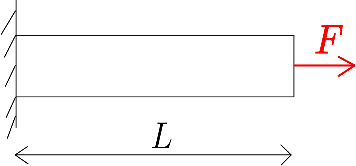
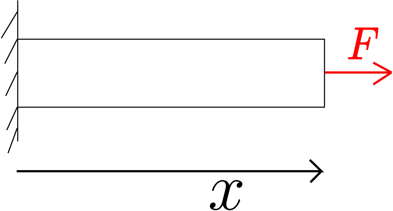
Let us start with a simple example which we have come across during our schooldays. Think of a horizontal
bar subjected to a force \(F\) as shown in Figure 5.1.
If its original length is \(L\) and the final length is \(l\), then we say that the strain generated in the bar is
This particular strain is called longitudinal strain (\(\epsilon \)) and is expressed mathematically as follows: \begin {equation} \label {5_longitudinal_strain_formula} \epsilon =\frac {l-L}{L}=\frac {\Delta L}{L}. \end {equation} We have one strain value for the whole bar and hence it can also be thought of as the bar’s global strain. Let us consider another example in which we have a bar hanging vertically under its own weight as shown in Figure 5.2.
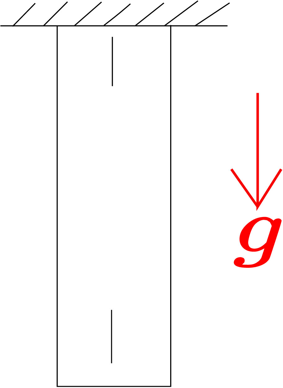
Let us think about the change in length of small line elements at two locations: one near the clamped end and the other near the other end of the bar (see Figure 5.2). It is observed that the line element near the clamped end undergoes a much larger change in length compared to the other line element. This shows that the change in length is different for different line elements across the length of the bar. We can thus define the strain at a particular location as the local strain.∗ This implies that, just like stress, strain also varies in the body.
Let us consider an arbitrarily shaped body (which need not look like a bar) subjected to an external distributed load as shown in Figure 5.3.
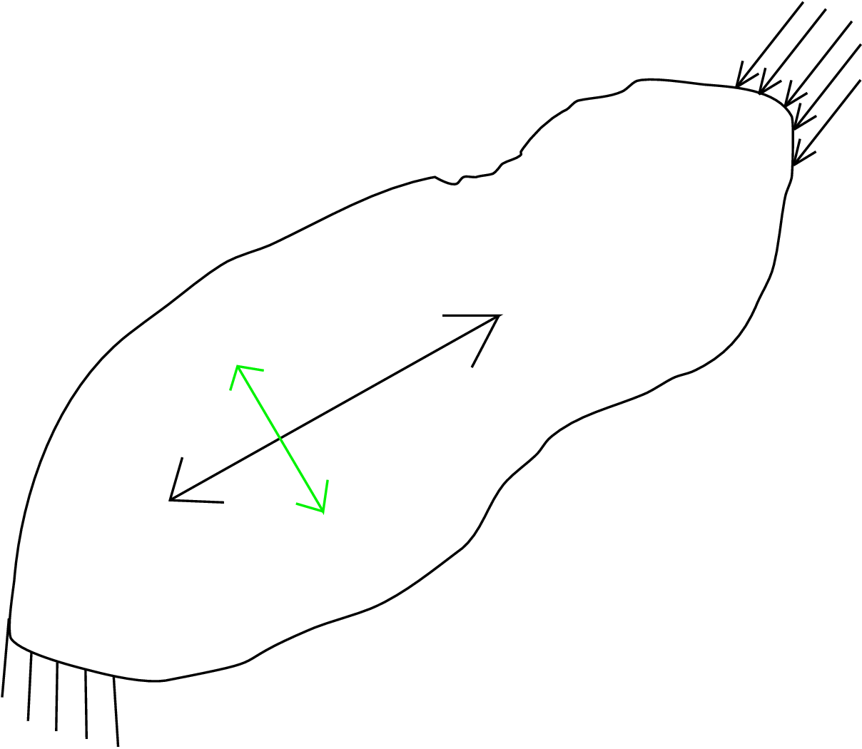
We want to find longitudinal strain at an arbitrary point in the body. In the two examples considered earlier, we had simply considered the change in length along the length of the bar to obtain longitudinal strain. But, here there is no such unique direction as in a bar and the body is, in fact, undergoing change in length or size in all directions - two such directions are shown in Figure 5.3 emanating from a point in the body.
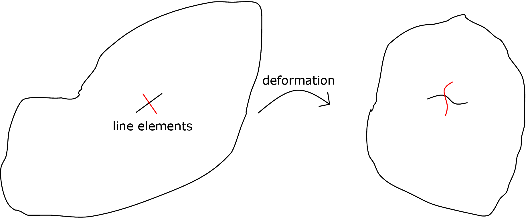
There are, in fact, infinite line elements emanating from this point.† As the body deforms, these line elements undergo change in shape and size as shown in Figure 5.4. However, if we assume the original/undeformed line elements passing through the point of interest to be infinitesimally small, the deformed curves can be approximated as straight lines too. This assumption helps in deriving a general formula for strain as we shall see later. Assuming line elements to be infinitesimally small also allows us to obtain longitudinal strain at a point in the body: if the line elements were of finite length, the longitudinal strain obtained would not correspond to a point but to the small region of the body in which the line element lies. As we have infinite line elements at every point in the body, we can associate infinite longitudinal strains at that point. So, longitudinal strain depends on two factors: the point at which we are measuring the strain and the line element that we choose at that point. Mathematically, we can define a line element at a point by its orientation/direction (denoted by \(\underline {n}\)). So, the longitudinal strain can be denoted by \(\epsilon (\underline {x},\underline {n})\). We should recall here that traction was also denoted by \(\underline {t}(\underline {x},\underline {n})\). The vector \(\underline {n}\) there denoted surface normal but in case of strain, \(\underline {n}\) denotes the line element direction.
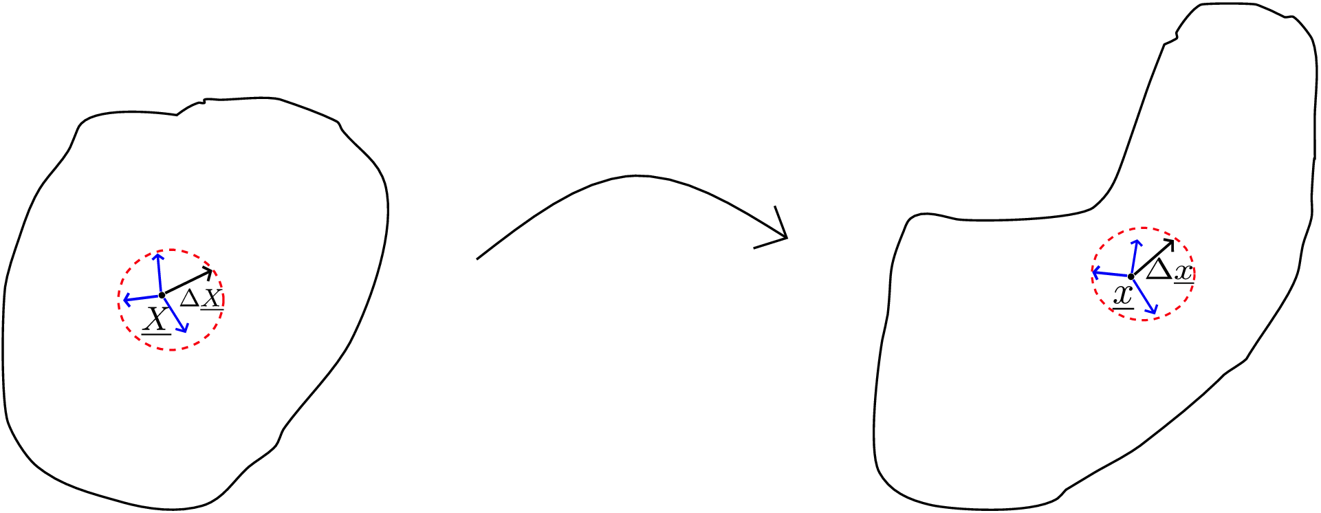
When a body gets deformed, every point in the body undergoes some displacement. Let us think of a reference configuration of the body relative to which we would measure the displacement of a point (see Figure 5.5).
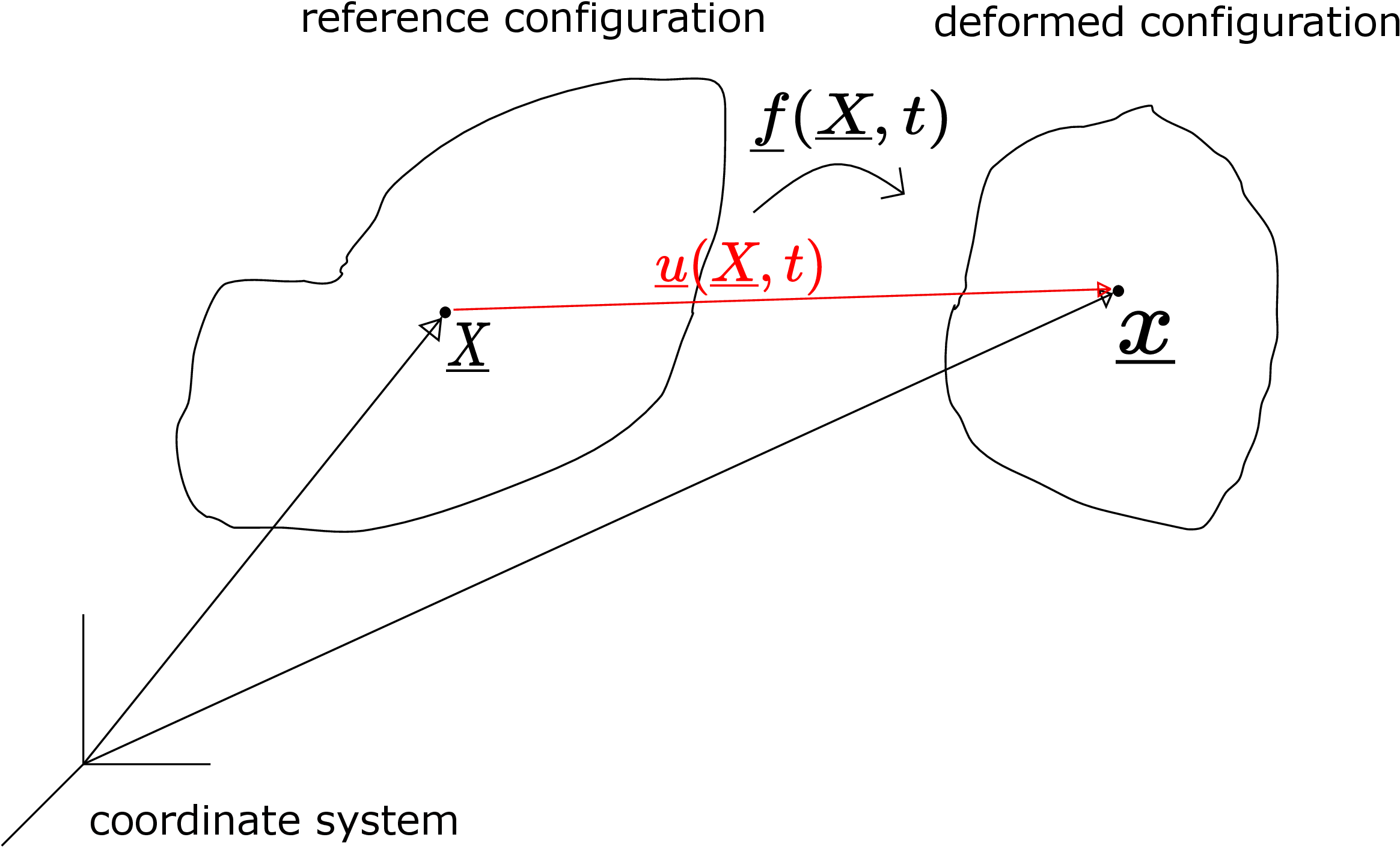
This reference configuration could be the configuration of the body at time \(t=0\) or the configuration when there is no load acting on the body or any other convenient configuration. The deformed configuration is shown on the right in Figure 5.5. We also define a coordinate system. The position vector of any point in the reference configuration is denoted by \(\underline {X}\). This point (which is also called a material point) displaces to the point \(\underline {x}\) in the deformed configuration. In fact, every point in the reference configuration has a corresponding point in the deformed configuration and we can think of a function which relates corresponding points in the two configurations. We denote this function by \(\underline {f}\) whose domain is the position vector of all the points in the reference configuration. The function returns deformed configuration of the body which typically changes with time. The position \(\underline {x}\) of a point in the deformed configuration can then be mathematically written as \begin {equation} \label {5_final_position_vector} \underline {x}=\underline {f}(\underline {X},t). \end {equation} Note that \(\underline {f}\) is a vector function since it has to return the deformed position vector. In component form, equation \eqref{5_final_position_vector} can also be written as follows: \begin {equation} \begin {bmatrix} x_1\\ x_2\\ x_3 \end {bmatrix}= \begin {bmatrix} f_1(X_1,X_2,X_3,t)\\ f_2(X_1,X_2,X_3,t)\\ f_3(X_1,X_2,X_3,t) \end {bmatrix}. \end {equation} Note that each component of \(\underline {f}\) is a function of all components of \(\underline {X}\), i.e., (\(X_1,X_2,X_3\)) and \(t\). The displacement of a point (denoted by \(\underline {u}\)) is then given by the vector from the reference position to the deformed position as shown by the red line in Figure 5.5. Mathematically, we say that this displacement \(\underline {u}\) depends on the point we are considering in the reference configuration as well as time. Thus, we have
With these notations introduced, let us now relate the line elements in reference and deformed configurations.
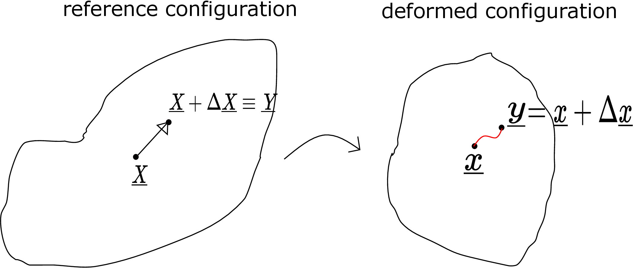
Let us look at the reference and deformed configurations of the body again as shown in Figure 5.6 and consider two points \(\underline {X}\) and \(\underline {Y}\) (\(\underline {X}+\Delta \underline {X}\)) very close to each other in the reference configuration. We are interested in the line element that joins these two points. As mentioned earlier, the material present on this line forms the material line element. After deformation, point \(\underline {X}\) goes to \(\underline {x}\) while \(\underline {Y}\) goes to \(\underline {y}\). In general, the deformed line element need not be a straight line but when the initial line segment is small enough, the deformed curve will be very similar to a straight line. In further analysis, we’ll let \(\Delta \underline {X}\) approach zero and so this assumption of deformed line element being straight will be valid in our analysis. In letting \(\Delta \underline {X}\rightarrow 0\), we also ensure that we find the strain at point \(\underline {X}\) itself. We then write the point \(\underline {y}\) as \(\underline {x}+\Delta \underline {x}\). The unit vector direction for the initial line element is given by
Finally, using equation \eqref{5_longitudinal_strain_formula}, the longitudinal strain at point \(\underline {X}\) for the line element along direction \(\underline {n}\) is given by \begin {equation} \epsilon (\underline {X},\underline {n})=\lim _{\vert \vert \Delta \underline {X}\vert \vert \to 0} \frac {\vert \vert \Delta \underline {x}\vert \vert -\vert \vert \Delta \underline {X}\vert \vert }{\vert \vert \Delta \underline {X}\vert \vert } \end {equation} The vector \(\Delta \underline {x}\) can be rewritten using equation \eqref{5_final_position_vector} as follows:
Let us now use Taylor’s expansion to expand \(\underline {f}(\underline {X}+\Delta \underline {X})\). As \(\Delta \underline {X}\) has got three components: \(\Delta {X}_1\Delta {X}_2,\Delta {X}_3\), the Taylor’s expansion will involve derivatives with respect to all the components, i.e., \begin {equation} \Delta \underline {x}=\underbrace {\underline {f}(\underline {X})+\frac {\partial \underline {f}}{\partial X_1}(\underline {X})\Delta X_1+\frac {\partial \underline {f}}{\partial X_2}(\underline {X})\Delta X_2+\frac {\partial \underline {f}}{\partial X_3}(\underline {X})\Delta X_3+...}_{\text {Taylor's expansion}} -\underline {f}(\underline {X}). \end {equation} We can also write the above in a compact form as shown below: \begin {equation} \Delta \underline {x}= \begin {bmatrix} \dfrac {\partial \underline {f}}{\partial X_1}& \dfrac {\partial \underline {f}}{\partial X_2}& \dfrac {\partial \underline {f}}{\partial X_3} \end {bmatrix} \begin {bmatrix} \Delta X_1\\ \Delta X_2\\ \Delta X_3 \end {bmatrix}+\frac {\partial ^2\underline {f}}{\partial X_1\partial X_1}\frac {\Delta X_1^2}{2}+\frac {\partial ^2\underline {f}}{\partial X_1\partial X_2}\Delta X_1\Delta X_2+.... \end {equation} Two higher order terms are shown to understand the pattern: we can see that both these terms have derivatives multiplied to expressions that are proportional to the square of magnitude of \(\Delta \underline {X}\) (\(\vert \vert \Delta \underline {X}\vert \vert ^2=\Delta X_1^2+\Delta X_2^2+\Delta X_3^2\)). So, all the higher order terms can be clubbed together as O(\(\vert \vert \Delta \underline {X}\vert \vert ^2\)) terms. Here ‘O(\(\cdot \))’ notation (pronounced big-oh) implies that the terms are of the same order, i.e.,‡ \begin {equation} lim_{\vert \vert \Delta \underline {X}\vert \vert \rightarrow 0}\frac {O(\vert \vert \Delta \underline {X}\vert \vert )^2}{\vert \vert \Delta \underline {X}\vert \vert ^2}= \text {a finite number}. \end {equation} Finally, we can write the following in matrix form: \begin {equation} \label {5_before_gradient} [\Delta \underline {x}]= \begin {bmatrix} \Delta x_1\\ \Delta x_2\\ \Delta x_3 \end {bmatrix}= \begin {bmatrix} \dfrac {\partial {f}_1}{\partial X_1}& \dfrac {\partial {f}_1}{\partial X_2} &\dfrac {\partial {f}_1}{\partial X_3}\\ \dfrac {\partial {f}_2}{\partial X_1}& \dfrac {\partial {f}_2}{\partial X_2} &\dfrac {\partial {f}_2}{\partial X_3}\\ \dfrac {\partial {f}_3}{\partial X_1}& \dfrac {\partial {f}_3}{\partial X_2} &\dfrac {\partial {f}_3}{\partial X_3} \end {bmatrix} \begin {bmatrix} \Delta X_1\\ \Delta X_2\\ \Delta X_3 \end {bmatrix} +O(\vert \vert \Delta \underline {X}\vert \vert ^2). \end {equation} Let us recall the definition of the gradient of a general vector quantity \(\underline {f}\), i.e.,
It turns out to be a second order tensor. Its matrix form in (\(\underline {e}_1\), \(\underline {e}_2\), \(\underline {e}_3\)) coordinate system is \(\begin {bmatrix}\underline {\underline {F}}\end {bmatrix}\) whose components are given by \(F_{ij}=\frac {\partial f_i}{\partial X_j}\). It is this matrix which is also appearing in equation \eqref{5_before_gradient} above. We can recall from the first chapter that the tensor form of a matrix-column multiplication is just the second order tensor corresponding to the matrix multiplied by the vector corresponding to the column. Thus, we can also write equation \eqref{5_before_gradient} in tensor form as follows: \begin {equation} \Delta \underline {x}=\underline {\underline {F}}~ \Delta \underline {X}+O(\vert \vert \Delta \underline {X}\vert \vert ^2). \end {equation} The vector function \(\underline {f}\) is called the deformation map and \(\underline {\underline {F}}\) the deformation gradient tensor. The above equation is very important since it relates the material line element \(\Delta \underline {X}\) at a point \(\underline {X}\) in the reference configuration to the corresponding deformed line element \(\Delta \underline {x}\) at \(\underline {x}\) in the deformed configuration.
Once we have the expression for \(\Delta \underline {x}\), we can express the square of final length (\(l^2\)) of a line element as
Note that all the higher order terms here are clubbed together as \(O(\vert \vert \Delta \underline {X}\vert \vert ^3)\): this is because \(\underline {\underline {F}}\Delta \underline {X}\) is an \(O(\vert \vert \Delta \underline {X}\vert \vert )\) which when dotted with an \(O(\vert \vert \Delta \underline {X}\vert \vert ^2)\) term results in an \(O(\vert \vert \Delta \underline {X}\vert \vert ^3)\) term.§ Similarly, the square of reference length (\(L^2\)) of a line element can be written as \begin {equation} L^2=\Delta \underline {X} \cdot \Delta \underline {X}. \end {equation} The square of stretch (\(\lambda ^2\)) in the line element then becomes
We can write \(\Delta \underline {X}\cdot \Delta \underline {X}\) as \(\vert \vert \Delta \underline {X}\vert \vert ^2\). Also, \(O(\vert \vert \Delta \underline {X}\vert \vert ^3)\) term when divided by \(\vert \vert \Delta \underline {X}\vert \vert ^2\) gives an \(O(\vert \vert \Delta \underline {X}\vert \vert )\) term. This finally yields \begin {equation} \lambda ^2=\Bigg (\underline {\underline {F}}\frac {\Delta \underline {X}}{\vert \vert \Delta \underline {X}\vert \vert }\Bigg )\cdot \Bigg (\underline {\underline {F}}\frac {\Delta \underline {X}}{\vert \vert \Delta \underline {X}\vert \vert }\Bigg )+O(\vert \vert \Delta \underline {X}\vert \vert ). \end {equation} Using equation \eqref{5_line_direction}, we can further write the above expression as \begin {equation} \label {5_lambda_deformation_gradient} \lambda ^2(\underline {X},\underline {n})=\underline {\underline {F}}\,\underline {n}\cdot \underline {\underline {F}}\,\underline {n}+O(\vert \vert \Delta \underline {X}\vert \vert ). \end {equation} Our final aim is to express the above formula in terms of displacement. So, we need to somehow write \(\underline {\underline {F}}\) in terms of the displacement. We begin with \begin {equation} \underline {f}=\underline {x}=\underline {X}+\underline {u}\Rightarrow f_i= X_i+ u_i. \end {equation} To find \(\underline {\underline {F}}\), we need the derivatives of \(f\), i.e.,
This is because \(X_i\)’s are independent coordinates in the reference configuration: the derivative of a component with respect to the same component will give 1 otherwise it will be 0. The tensor form of the above equation would be \begin {equation} \underline {\underline {F}}=\underline {\nabla }\,\underline {f}=\underline {\underline {I}}+\underline {\nabla }\,\underline {u} \end {equation} where the tensor \(\underline {\nabla }\,\underline {u}\) is called the displacement gradient tensor. Substituting above equation in equation \eqref{5_lambda_deformation_gradient}, we get \begin {equation} \label {lambda_before_identity} \lambda ^2(\underline {X},\underline {n})=\Big (\underline {\underline {I}}+\underline {\nabla }\,\underline {u}\Big )\underline {n} \cdot \Big (\underline {\underline {I}}+\underline {\nabla }\,\underline {u}\Big )\underline {n}+O(\vert \vert \Delta \underline {X}\vert \vert ). \end {equation} We then use the following identity: \begin {equation} \label {identity} \underline {\underline {A}}\,\underline {a}\cdot \underline {b}=\underline {a}\cdot \underline {\underline {A}}^T\underline {b} \end {equation} which yields
Here we used \(\underline {\underline {I}}^T=\underline {\underline {I}}\) since an identity tensor is a symmetric tensor. We finally need to reduce the length of the line element in the reference configuration to zero in order to obtain the local value of stretch, i.e., we have to take the limit of \(\vert \vert \Delta \underline {X}\vert \vert \to 0\). The \(O(\vert \vert \Delta \underline {X}\vert \vert )\) then vanishes.¶ We finally have \begin {equation} \label {5_lambda} \lambda ^2(\underline {X},\underline {n})=\underline {n}\cdot \Big [\underline {\underline {I}}+\underline {\nabla }\,\underline {u}+\underline {\nabla }\,\underline {u}^T+\underline {\nabla }\,\underline {u}^T\underline {\nabla }\,\underline {u}\Big ]\underline {n}. \end {equation} We can simplify this even further. In this course, we will only be working with displacements such that their gradients are very small, i.e., \begin {equation} \Bigg \vert \frac {\partial u_i}{\partial x_j}\Bigg \vert \ll 1. \end {equation} The term \(\underline {\nabla }\,\underline {u}^T\underline {\nabla }\,\underline {u}\) in \eqref{5_lambda}, when written in matrix form, has two matrices multiplied and each of them contains derivatives of \(u\). So, the product matrix will have components which are quadratic combinations of displacement gradients. As the displacement gradients themselves are very small, their quadratic combinations will be even smaller. Hence, the term \(\underline {\nabla }\,\underline {u}^T\underline {\nabla }\,\underline {u}\) becomes insignificant compared to \(\underline {\nabla }\,\underline {u}\) and can be neglected. One may think that as \(\underline {\nabla }\,\underline {u}\) itself is much smaller than 1, it should also be neglected. But, in the definition for strain, it will turn out to be the most significant term (see equation \eqref{5_longitudinal_strain_final} below). The idea is that we keep the most significant term while neglecting the other less significant terms. So, we have the following expression:
Having obtained longitudinal stretch, the longitudinal strain then becomes
We can now use binomial expansion to simplify the square root term which yields the following simpler tensor formula for longitudinal strain at a point in a prescribed direction
Here again, we have dropped quadratic and higher order terms from binomial expansion for the same reason as earlier.
If the line element direction \(\underline {n}\) is taken to be \(\underline {e}_1\), the matrix form of \eqref{5_longitudinal_strain_final} in (\(\underline {e}_1\), \(\underline {e}_2\), \(\underline {e}_3\)) coordinate system will be
Similar analysis can be done for \(\underline {n}=\underline {e}_2,~\underline {e}_3\) leading to \begin {equation} \label {5_longitudinal_e1_e2_e3} \epsilon (\underline {X},\underline {e}_2)=\frac {\partial u_2}{\partial X_2},\quad \epsilon (\underline {X},\underline {e}_3)=\frac {\partial u_3}{\partial X_3}. \end {equation} We can compare the strains obtained above with what we have seen during our schooldays. For example, consider the straight bar that we had seen at the start of this chapter (see Figure 5.7).
The origin of the coordinate system is at the clamped end and the bar is lying along \(x\)-axis. If we say the bar gets uniformly stretched by \(\lambda \) or the bar gets axially strained by \(\epsilon \), the displacement of the bar will be given by \begin {equation} \label {straight_displacement} u=(\lambda -1)x = \epsilon x. \end {equation} This is because displacement will be zero at the clamped end and then increases linearly along the length of the bar. When we calculate \(\dfrac {\partial u}{\partial x}\) from the above equation, we get \begin {equation} \frac {\partial u}{\partial x}=\lambda -1=\epsilon . \end {equation} So, we can see that our general formula for strain in \eqref{5_longitudinal_strain_final} yields the correct strain value. This completes our discussion for longitudinal strain in a general three-dimensional body.
We have another type of strain which measures the change in angle between two perpendicular line elements (also see Figure 5.8). Such a measure of strain is called shear strain. After the body gets deformed, the angle between those line elements need not remain \(90^\circ \). If this angle after deformation is denoted by \(\beta \), the change in angle (denoted by \(\gamma \)) will be \begin {equation} \label {5_change_in_angle} \gamma =90^\circ -\beta \end {equation} which is the shear strain at this point in the body. It is responsible for generating distortion in a body leading to change in its shape whereas longitudinal strain changes the size of the body. For example, a rectangular body can become a parallelogram (keeping its area unchanged) due to shear strain as the angle between its edges changes. Our goal is to find the formula for shear strain just as we found one for longitudinal strain. Consider a body before and after deformation as shown in Figure 5.8.
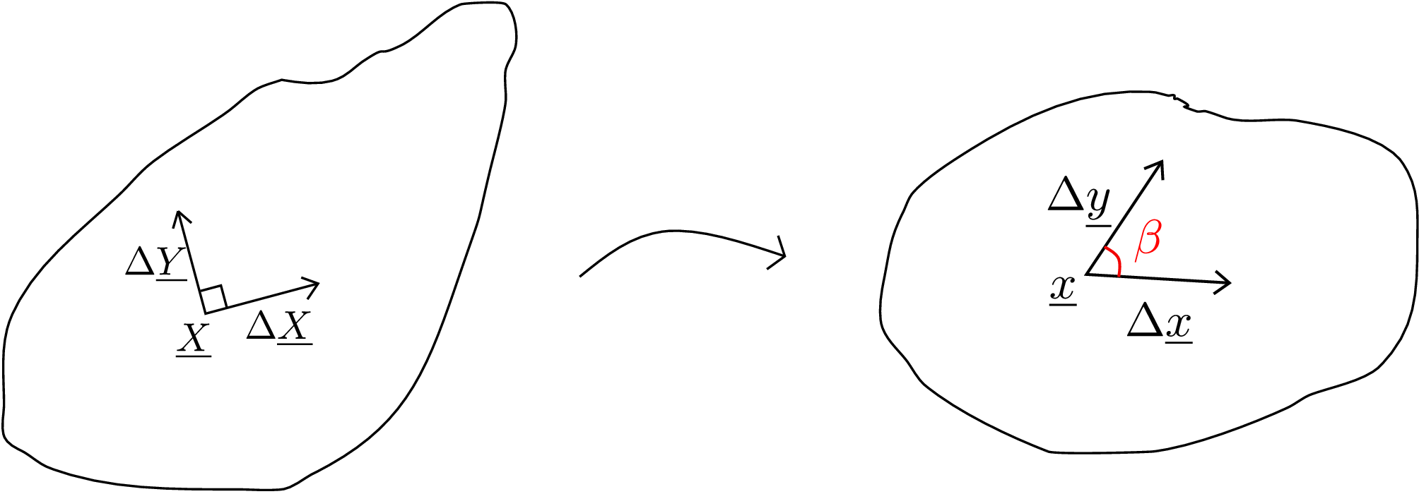
At the point of interest \(\underline {X}\) in the reference configuration, we identify two perpendicular line elements \(\Delta \underline {X}\) and \(\Delta \underline {Y}\). After deformation of the body, \(\Delta \underline {X}\) becomes \(\Delta \underline {x}\) and \(\Delta \underline {Y}\) becomes \(\Delta \underline {y}\).ʺ Let the unit vectors along line elements \(\Delta \underline {X}\) and \(\Delta \underline {Y}\) be denoted by \(\underline {n}\) and \(\underline {m}\) respectively, i.e., \begin {equation} \label {5_directions_line_elements} \underline {n}=\frac {\Delta \underline {X}}{\vert \vert \Delta \underline {X}\vert \vert },\quad \underline {m}=\frac {\Delta \underline {Y}}{\vert \vert \Delta \underline {Y}\vert \vert }. \end {equation} In general, the two line elements undergo stretching and the angle between them also changes. We have already derived the expression for deformed line element in terms of the deformation gradient tensor \(\underline {\underline {F}}\) according to which
Similar to the case of longitudinal strain, we keep the higher order terms because we don’t know if they are significant or not. The angle between these two line elements in the deformed configuration (denoted by \(\beta \)) will be given by \begin {equation} cos\beta =\frac {\Delta \underline {x}\cdot \Delta \underline {y}}{\vert \vert \Delta \underline {x}\vert \vert \,\vert \vert \Delta \underline {y}\vert \vert }. \end {equation} Let us substitute equation \eqref{5_deformed_line_elements} in the numerator above and express the terms in denominator using stretch, i.e.,
Here \(O(\cdot )\) terms vanish in the limit of length of both the line elements going to zero. Furthermore, as \(\epsilon (\underline {X},\underline {n})\) and \(\epsilon (\underline {X},\underline {m})\) are along directions \(\underline {n}\) and \(\underline {m}\) respectively, we denote them as \(\epsilon _{nn}\) and \(\epsilon _{mm}\), i.e.,
We can now apply binomial expansion formula because we know that longitudinal strains are very small compared to 1 (they are of the order of displacement gradient components), i.e., \begin {equation} cos\beta \approx (\underline {\underline {F}}\,\underline {n}\cdot \underline {\underline {F}}\,\underline {m})\,(1-\epsilon _{nn})(1-\epsilon _{mm}) + O(\vert \vert \underline {\nabla }\,\underline {u}\vert \vert ^2). \end {equation} Upon further expressing the deformation gradient tensor in terms of displacement gradient, we have
We can again drop \(\underline {\nabla }\,\underline {u}^T\underline {\nabla }\,\underline {u}\) term as we had done in the longitudinal strain formulation leading to
As \(\underline {m}\) and \(\underline {n}\) are perpendicular, their dot product will be zero. Also, as longitudinal strains are of the order of \(\vert \vert \underline {\nabla }\,\underline {u}\vert \vert \), their multiplication with other terms will generate quadratic or higher order terms in \(\vert \vert \underline {\nabla }\,\underline {u}\vert \vert \) and hence are neglected. Thus, we finally have \begin {equation} cos\beta =\Big [\big (\underline {\nabla }\,\underline {u}+\underline {\nabla }\,\underline {u}^T\big )\underline {m}\Big ]\cdot \underline {n}. \end {equation} Using basic trigonometry and equation \eqref{5_change_in_angle}, we can then write
As the gradients of displacement are very small, the RHS of the above equation is very small (usually of the order of \(10^{-2}\)). Therefore \(sin(\gamma )\) also becomes very small and can be replaced with just \(\gamma \), i.e., \begin {equation} \label {5_final_shear_strain} \boxed {\gamma =\big (\underline {\nabla }\,\underline {u}+\underline {\nabla }\,\underline {u}^T\big )\underline {m}\cdot \underline {n}} \end {equation} We can notice that the above formula for shear strain depends on the directions of the two line elements. Thus, at a point in a body, we will have different values of shear strain for different pairs of perpendicular line elements. Let us write the matrix form of \(\dfrac {1}{2}\big (\underline {\nabla }\,\underline {u}+\underline {\nabla }\,\underline {u}^T\big )\) in (\(\underline {e}_1,\underline {e}_2,\underline {e}_3\)) coordinate system, i.e., \begin {equation} \label {5_half_gradu+gradu_transpose_matrix} \begin {bmatrix} \frac {1}{2}\big (\underline {\nabla }\,\underline {u}+\underline {\nabla }\,\underline {u}^T\big ) \end {bmatrix}_{(\underline {e}_1,\underline {e}_2,\underline {e}_3)}= \begin {bmatrix} \dfrac {\partial u_1}{\partial X_1} & \dfrac {1}{2}\bigg (\dfrac {\partial u_1}{\partial X_2}+\dfrac {\partial u_2}{\partial X_1}\bigg ) & \dfrac {1}{2}\bigg (\dfrac {\partial u_1}{\partial X_3}+\dfrac {\partial u_3}{\partial X_1}\bigg )\\\\ \dfrac {1}{2}\bigg (\dfrac {\partial u_1}{\partial X_2}+\dfrac {\partial u_2}{\partial X_1}\bigg ) & \dfrac {\partial u_2}{\partial X_2} & \dfrac {1}{2}\bigg (\dfrac {\partial u_2}{\partial X_3}+\dfrac {\partial u_3}{\partial X_2}\bigg )\\\\ \dfrac {1}{2}\bigg (\dfrac {\partial u_1}{\partial X_3}+\dfrac {\partial u_3}{\partial X_1}\bigg ) & \dfrac {1}{2}\bigg (\dfrac {\partial u_2}{\partial X_3}+\dfrac {\partial u_3}{\partial X_2}\bigg ) & \dfrac {\partial u_3}{\partial X_3} \end {bmatrix}. \end {equation} Being a symmetric tensor, its matrix form also turns out to be symmetric.∗∗ We can see upon comparing from equation \eqref{5_longitudinal_e1_e2_e3} that the diagonal elements of the above matrix give us longitudinal strains along \(\underline {e}_1\), \(\underline {e}_2\) and \(\underline {e}_3\) directions. To understand the significance of the off-diagonal elements, let us choose the two line element directions \(\underline {n}\) and \(\underline {m}\) in equation \eqref{5_final_shear_strain} to be \(\underline {e}_1\) and \(\underline {e}_2\) respectively. We denote the shear strain for this case as \(\gamma _{12}\) because of the directions chosen which equals
When worked out using the matrix form, it turns out to be twice of the off-diagonal term in second row and first column of \eqref{5_half_gradu+gradu_transpose_matrix}, i.e.,
We can thus conclude that in matrix \eqref{5_half_gradu+gradu_transpose_matrix}, the off-diagonal components represent half the shear strains.
Let us visualize the above expression for shear strain. Consider the body shown in Figure 5.9
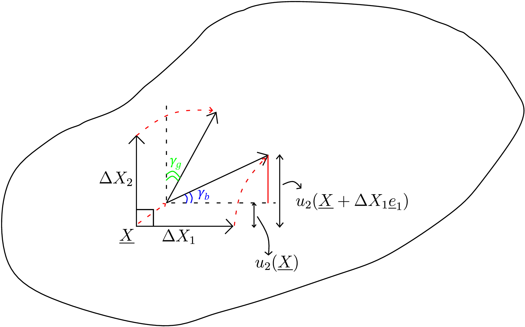
and try to obtain shear strain at point \(\underline {X}\). We choose the line elements along \(\underline {e}_1\) and \(\underline {e}_2\) in the reference configuration having their lengths \(\Delta X_1\) and \(\Delta X_2\) respectively. After deformation, the point \(\underline {X}\) as well as the line elements will shift to new positions as shown in the figure. We have also drawn horizontal and vertical axes (shown by dotted lines) at the deformed position \(\underline {x}\). The total change in angle between the two line elements will be the sum of the angles shown in blue and green. We call the angle shown in blue as \(\gamma _b\) and the angle shown in green as \(\gamma _g\). Thus \begin {equation} \label {5_total_alpha} \gamma _{12}=\gamma _b+\gamma _g. \end {equation} Let’s find \(\gamma _b\) first. Consider the right-angled triangle containing angle \(\gamma _b\). The red distance there is the difference in \(y\)-displacement of the tip and vertex of the initially horizontal line element. The length of the base of this right angled triangle will be approximately \(\Delta X_1\) since the longitudinal strain is much smaller than 1. Thus, the angle \(\gamma _b\) will be given by \begin {equation} \gamma _b= tan^{-1}\left (\frac {u_2(\underline {X}+\Delta X_1~\underline {e}_1)-u_2(\underline {X})}{\Delta X_1}\right )\approx \frac {u_2(\underline {X}+\Delta X_1~\underline {e}_1)-u_2(\underline {X})}{\Delta X_1}. \end {equation} Finally, to find this angle at point \(\underline {X}\) itself, \(\Delta X_1\) should tend to zero, i.e.,
By similar analysis, we can find \(\gamma _g\), i.e.,
Using equation \eqref{5_total_alpha}, we then get \begin {equation} \gamma _{12}=\frac {\partial u_2}{\partial X_1}+\frac {\partial u_1}{\partial X_2}. \end {equation} Thus, we have realized the physical significance of this expression for shear strain: it is the sum of the rotation of the two line elements from their initial orientation.
Let us consider the following displacement function:
and understand the underlying deformation. After deformation, the position vector of a typical point in the body changes as follows:
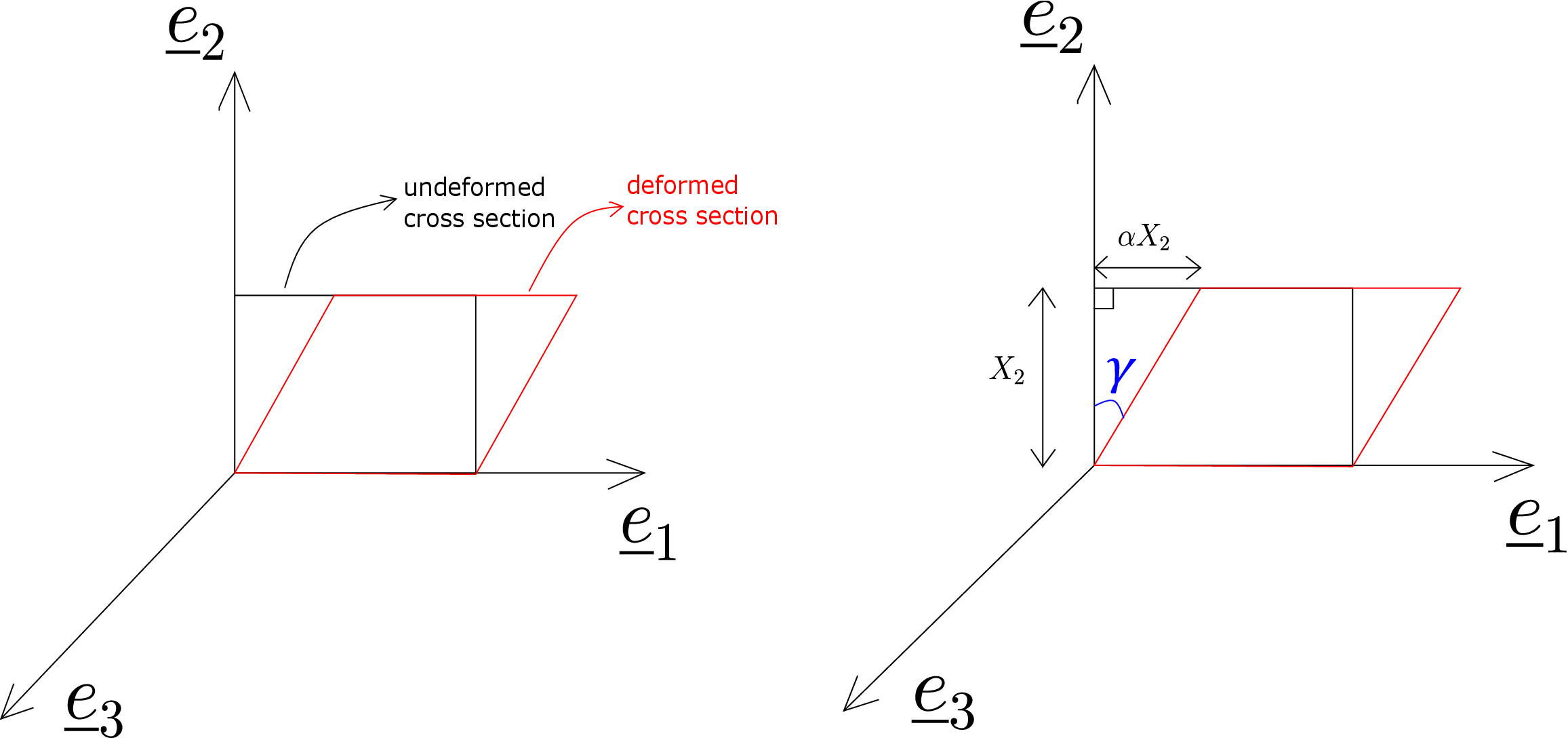
Think of a rectangular slice/cross-section of the body in \(\underline {e}_1-\underline {e}_2\) plane in its reference configuration (shown in black in Figure 5.10). This slice deforms to a parallelogram according to \eqref{5_displacement_function} as shown in red in the figure: it induces change in angle between its two perpendicular edges. Therefore, the displacement prescribed by equation \eqref{5_displacement_function} is also called shear displacement. To measure the amount of shear, we can directly notice from Figure 5.10b that
Alternatively, using the formula for shear, we can also see
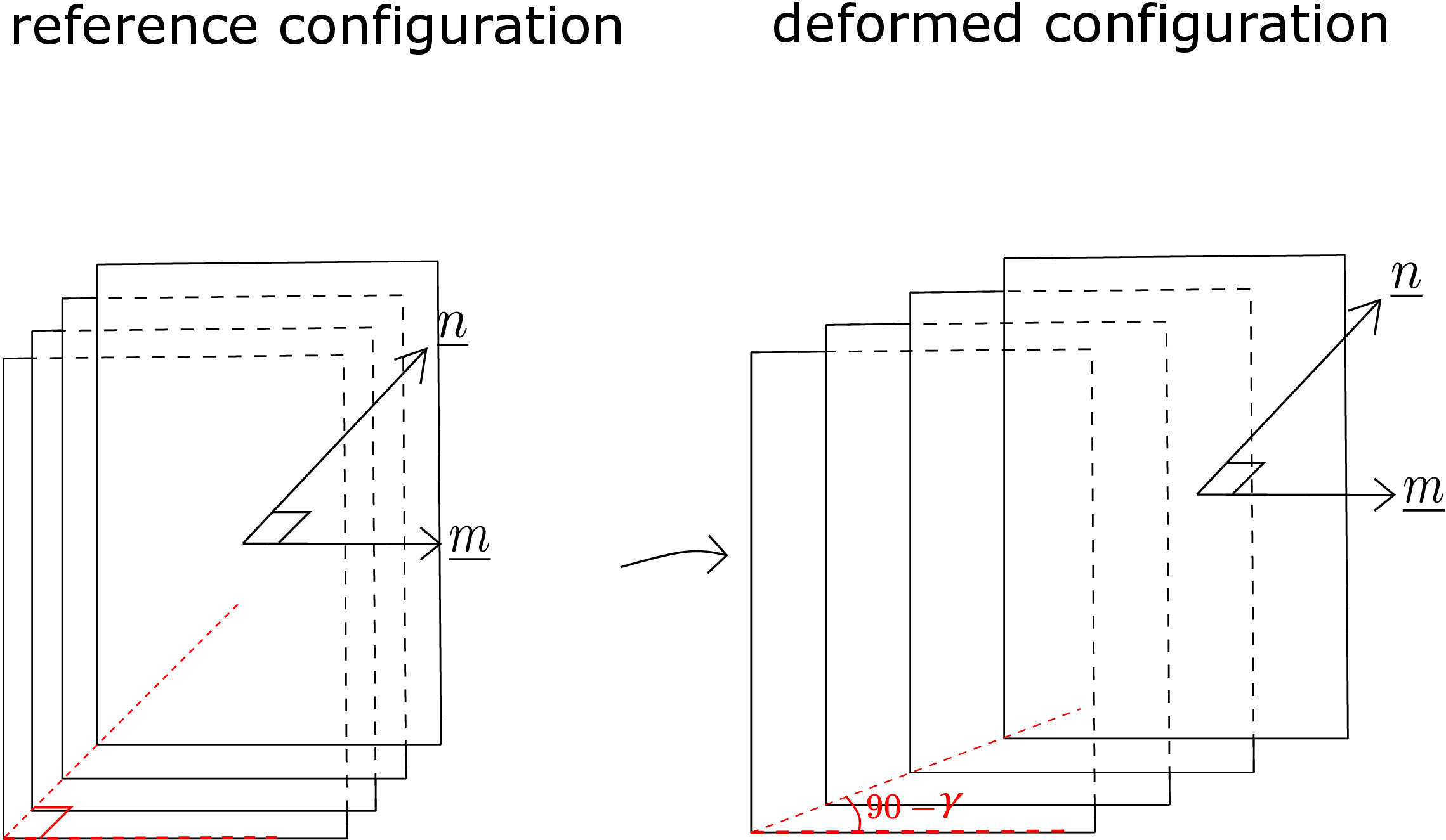
Let us now imagine a plane section of the body lying in (\(\underline {e}_1-\underline {e}_3\)) plane. This plane has constant \(X_2\)-coordinate. According to \eqref{5_displacement_function}, all points in this plane displace by same amount along \(\underline {e}_1\) direction. Hence, such planes do not deform but simply rigidly translate along \(\underline {e}_1\) by \(\alpha X_2\). One can, in fact, think of infinite such planes all parallel to each other having different \(X_2\) coordinate but each plane having the same \(X_2\) coordinate for all its points (also see Figure 5.11). The plane having \(X_2=0\) (lowermost plane in Figure 5.11) will have the same reference and deformed position. However, higher the \(X_2\) coordinate of a plane, higher is its drift/translation in \(\underline {e}_1\) direction. This can be visualized as sliding of a pack of cards (see Figure 5.11b). This is an alternate physical interpretation of shearing: sliding of parallel planes in a direction perpendicular to the plane normal. In the particular example under consideration, sliding is along \(\underline {e}_1\) direction which is perpendicular to \(\underline {e}_2\) (the plane normal). We can also let the planes slide in an arbitrary direction perpendicular to \(\underline {e}_2\) (other than \(\underline {e}_1\)) and that will also be shear. The angle \(\gamma \) in figures 5.10b and 5.11b is the measure of intensity of sliding of parallel planes and equals the shear strain value.
Let us again consider a body being deformed as shown in Figure 5.12. As the body deforms, the volume of every small region (called local volume element) of the body also changes. We can therefore define a quantity called local volumetric strain because, in general, the change in volume per unit volume will be different at different parts in the body. Let us think of three line elements \(\Delta \underline {X}\), \(\Delta \underline {Y}\) and \(\Delta \underline {Z}\) forming a parallelepiped at the point of interest \(\underline {X}\) in the reference configuration as shown in Figure 5.12.
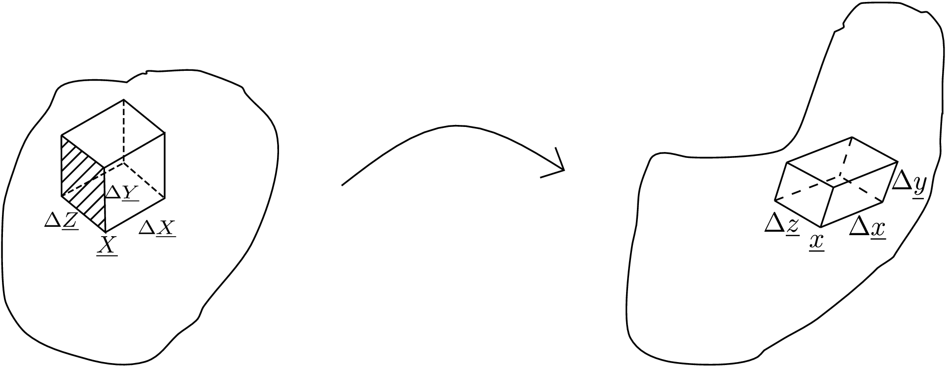
We should keep in mind that the sides of the parallelepiped are very small so that the parallelepiped lies in a tiny region near \(\underline {X}\). When the volume of this parallelepiped is shrunk to zero, we will be able to define local volumetric strain at point \(\underline {X}\) itself. Upon deformation, point \(\underline {X}\) goes to \(\underline {x}\) and the three line elements become \(\Delta \underline {x}\), \(\Delta \underline {y}\) and \(\Delta \underline {z}\) which again generate a parallelepiped. As the volume of a parallelepiped is given by scalar triple product of the three vectors forming its sides, the volume of the parallelepiped in the reference configuration (denoted by \(V\)) will be \begin {equation} V=\Delta \underline {X}\cdot (\Delta \underline {Y}\times \Delta \underline {Z}). \end {equation} Here the term \((\Delta \underline {Y}\times \Delta \underline {Z})\) gives the area formed by vectors \(\Delta \underline {Y}\) and \(\Delta \underline {Z}\) - the face of the parallelepiped corresponding to this is shaded in Figure 5.12. This face is considered to be the base of the parallelepiped. For this base, the height of the parallelepiped will be the component of \(\Delta \underline {X}\) along the shaded face’ normal. So, the volume is obtained by taking the dot product of the base area vector with \(\Delta \underline {X}\). Similarly, the volume of the parallelepiped in the deformed configuration (denoted by \(v\)) will be \begin {equation} v=\Delta \underline {x}\cdot (\Delta \underline {y}\times \Delta \underline {z}). \end {equation} The scalar triple product can also be realized as the determinant of a matrix whose columns are formed by the vectors involved in the scalar triple product. Thus, we can write
Substituting the below formula in \eqref{5_deformed_volume} \begin {equation} \Delta \underline {x}=\underline {\underline {F}}\Delta \underline {X}+O\big (\vert \vert \Delta \underline {X}\vert \vert ^2\big ), \end {equation} we get
We can simplify it further by using the following identity:
This implies that
Substituting this in \eqref{5_new_volume_before_trick} and further dividing by the reference volume, we get \begin {equation} \label {5_local_vol_strain} \frac {v}{V}=det\Big [\underline {\underline {F}}\Big ] + O\left (\vert \vert \Delta \underline {X}\vert \vert \right )+O\left (\vert \vert \Delta \underline {Y}\vert \vert \right )+O\left (\vert \vert \Delta \underline {Z}\vert \vert \right ). \end {equation} Upon substituting this in the below formula for volumetric strain \begin {equation} \label {5_longtudinal_strain_formula} \epsilon _V=\lim _{V\to 0}\bigg (\frac {v}{V}-1\bigg ), \end {equation} we finally obtain \begin {equation} \label {5_volumetric_strain_det_f} \epsilon _V=det\Big [\underline {\underline {F}}\Big ]-1. \end {equation} Let us now write the deformation gradient matrix in terms of displacement gradient components, i.e.,
To obtain its determinant, let us expand it in terms of first row, i.e.,
Finally, ignoring the higher order terms and using equation \eqref{5_volumetric_strain_det_f}, we get the following formula for local volumetric strain: \begin {equation} \boxed {\epsilon _V=\frac {\partial u_1}{\partial X_1}+\frac {\partial u_2}{\partial X_2}+\frac {\partial u_3}{\partial X_3}} \end {equation} We can notice that the RHS of this equation is equal to the trace†† of the displacement gradient matrix. Thus, we can also write
It should be noted that unlike longitudinal and shear strains, the volumetric strain turns out to be independent of what triplet of line elements is chosen at a point. Thus, the volumetric strain is unique at a point in a body.
Let us now look at the expressions of all the strains derived till now: \begin {alignat*} {2} \text {longitudinal strain }&:\,\epsilon _{nn}(\underline {X},\underline {n})&=&~\frac {1}{2}\Big (\underline {\nabla }\,\underline {u}+\underline {\nabla }\,\underline {u}^T\Big )\underline {n}\cdot \underline {n}\nonumber \\ \text {shear strain }&:\,\gamma _{mn}(\underline {X},\underline {n},\underline {m})&=&~2\bigg (\frac {1}{2}\Big (\underline {\nabla }\,\underline {u}+\underline {\nabla }\,\underline {u}^T\Big )\underline {n}\cdot \underline {m}\bigg )\nonumber \\ \text {volumetric strain }&:\,\epsilon _V(\underline {X})&=&~tr\bigg (\frac {1}{2}\Big (\underline {\nabla }\,\underline {u}+\underline {\nabla }\,\underline {u}^T\Big )\bigg ) \end {alignat*}
We can notice that the expressions for all the strains are dependent on the tensor \(\dfrac {1}{2}\Big (\underline {\nabla }\,\underline {u}+\underline {\nabla }\,\underline {u}^T\Big )\). This quantity is called the infinitesimal strain tensor which we will denote by \(\underline {\underline {\epsilon }}\). In matrix form in (\(\underline {e}_1,\underline {e}_2,\underline {e}_3\)) coordinate system, it becomes \begin {equation} \label {5_strain_matrix} \begin {bmatrix}\underline {\underline {\epsilon }}\end {bmatrix}=\begin {bmatrix} \dfrac {\partial u_1}{\partial X_1} & \dfrac {1}{2}\bigg (\dfrac {\partial u_2}{\partial X_1}+\dfrac {\partial u_1}{\partial X_2}\bigg ) & \dfrac {1}{2}\bigg (\dfrac {\partial u_3}{\partial X_1}+\dfrac {\partial u_1}{\partial X_3}\bigg )\\\\ \dfrac {1}{2}\bigg (\dfrac {\partial u_2}{\partial X_1}+\dfrac {\partial u_1}{\partial X_2}\bigg ) & \dfrac {\partial u_2}{\partial X_2} & \dfrac {1}{2}\bigg (\dfrac {\partial u_3}{\partial X_2}+\dfrac {\partial u_2}{\partial X_3}\bigg )\\\\ \dfrac {1}{2}\bigg (\dfrac {\partial u_3}{\partial X_1}+\dfrac {\partial u_1}{\partial X_3}\bigg ) & \dfrac {1}{2}\bigg (\dfrac {\partial u_3}{\partial X_2}+\dfrac {\partial u_2}{\partial X_3}\bigg ) & \dfrac {\partial u_3}{\partial X_3} \end {bmatrix}. \end {equation} The individual components of this matrix can also be written as follows: \begin {equation} \epsilon _{ij}=\frac {1}{2}\bigg (\frac {\partial u_i}{\partial X_j}+\frac {\partial u_j}{\partial X_i}\bigg ). \end {equation}
Let us again consider the reference and deformed configurations of a body. Our point of interest \(\underline {X}\) in the reference configuration gets mapped to the point \(\underline {x}\) in the deformed configuration as shown in Figure 5.13.
We have infinite line elements that one can think of at \(\underline {X}\) some of which are shown there. Any undeformed line element gets transformed to the deformed line element using the relation \(\Delta \underline {x}=\underline {\underline {F}}\Delta \underline {X}\) if the undeformed line element is small enough. We also know the relation between the deformation gradient tensor and the displacement gradient tensor which we can also write as follows:
The symmetric part of the displacement gradient tensor was defined as the strain tensor (\(\underline {\underline {\epsilon }}\)) earlier. We have further
denoted the anti-symmetric part of the displacement gradient tensor as \(\underline {\underline {W}}\). This decomposition allows us to write \begin {equation} \label {5_line_element_deformation_significance} \Delta \underline {x}=\underline {\underline {F}}\Delta \underline {X}=\underline {\underline {\epsilon }}~\Delta \underline {X}+(\underline {\underline {I}}+\underline {\underline {W}})~\Delta \underline {X}. \end {equation} This
representation for the deformed line element has a physical meaning associated to it. To see this, let us
again look at Figure 5.13 where a small region around \(\underline {X}\) is shown by the red dashed curve. The line
elements in this volume are transformed by multiplying \(\underline {\underline {F}}\) to them. According to the representation given in
equation \eqref{5_line_element_deformation_significance}, the first term \(\underline {\underline {\epsilon }}~\Delta \underline {X}\) is responsible for straining the
small volume around \(\underline {X}\), i.e., it generates longitudinal, shear and volumetric strains in this region. If the
displacement is such that the strain tensor \(\underline {\underline {\epsilon }}\) is \(\underline {\underline {0}}\) at a point, then there will be no strain of any kind in the
neighbourhood of that point. Stated differently, the line elements in a tiny volume around that point will
undergo no change in length or change in angle between them. The tiny volume will also retain its
volume. However, due to remaining terms in \eqref{5_line_element_deformation_significance}, we
will prove later that these line elements undergo rigid rotation. As \(\underline {\underline {W}}\) can vary from point to point, this
rigid rotation will be different at different points which is a bit difficult to visualize: the body being
deformable (not rigid), tiny volumes around different points of a body need not undergo same rigid rotation.
To prove that \(\underline {\underline {I}}+\underline {\underline {W}}\) is indeed responsible for local rotation, we first introduce a way to express rotation
tensor.
Suppose \(\underline {a}\) is a unit vector denoting the axis of rotation and \(\theta \) is the angle of rotation about this axis. Then, according
to Rodrigue’s formula, the rotation tensor is given by \begin {equation} \label {5_Rodrigues_general} \underline {\underline {R}}(\underline {a},\theta )=\underline {\underline {I}}\cos \theta +\underline {\underline {a}}~\sin \theta +\underline {a}\otimes \underline {a}~(1-\cos \theta ). \end {equation} Here \(\underline {\underline {a}}\) denotes the skew symmetric tensor corresponding to \(\underline {a}\).
This is a general formula for rotation which is valid even when the angle of rotation \(\theta \) is large. Let’s consider the case
when \(\theta \) is very small. We can then approximate the trigonometric functions using their Taylor’s expansion, i.e.,
Note that we have kept only the terms that are most significant. Substituting them in equation \eqref{5_Rodrigues_general}, we get
Thus, an arbitrarily small/infinitesimal rotation can be represented using the above formula which can now be compared with the expression \(\underline {\underline {I}}+\underline {\underline {W}}\) in \eqref{5_line_element_deformation_significance}. This proves that \(\underline {\underline {I}}+\underline {\underline {W}}\) indeed represents local infinitesimal rotation. Let \(\underline {w}\) denote the axial vector of \(\underline {\underline {W}}\). Then, upon comparing \(\underline {\underline {I}}+\underline {\underline {W}}\) with \eqref{5_small_rotation}, we conclude the following:
Let us now look at the matrix form of the skew symmetric tensor \(\underline {\underline {W}}\) in (\(\underline {e}_1,\underline {e}_2,\underline {e}_3\)) coordinate system:
The column form of axial vector of \(\underline {\underline {W}}\) will then be \begin {equation} \label {5_axial_general} \begin {bmatrix} \underline {w} \end {bmatrix}= \begin {bmatrix} \dfrac {1}{2}\bigg (\dfrac {\partial u_3}{\partial X_2}-\dfrac {\partial u_2}{\partial X_3}\bigg )\\\\ \dfrac {1}{2}\bigg (\dfrac {\partial u_1}{\partial X_3}-\dfrac {\partial u_3}{\partial X_1}\bigg )\\\\ \dfrac {1}{2}\bigg (\dfrac {\partial u_2}{\partial X_1}-\dfrac {\partial u_1}{\partial X_2}\bigg ) \end {bmatrix}. \end {equation} The magnitude of this vector is the angle of local rotation and the unit vector in its direction is the axis of local rotation.
Let us consider an example where our coordinate system is (\(\underline {e}_1,\underline {e}_2,\underline {e}_3\)) and the displacement components are given as follows:
We have assumed \(u_1\) and \(u_2\) components to be independent of the third coordinate and \(u_3\) is assumed to be zero. So, the strain matrix in this case according to \eqref{5_strain_matrix} will be
It has basically a \(2\times 2\) non-zero submatrix. This is also called the plane strain case since all the strains involving \(\underline {e}_3\) direction are zero. We can then obtain the axial vector corresponding to local rotation using equation \eqref{5_axial_general} to be \begin {equation} \label {5_e_3_axial_vector} \begin {bmatrix} \underline {w} \end {bmatrix}= \begin {bmatrix} 0\\ 0\\ \dfrac {1}{2}\bigg (\dfrac {\partial u_2}{\partial X_1}-\dfrac {\partial u_1}{\partial X_2}\bigg ) \end {bmatrix}. \end {equation} Let us now see how the above strain and rotation matrices act on the system. As the displacement is confined in \(\underline {e}_1-\underline {e}_2\) plane, we take two line elements in this plane
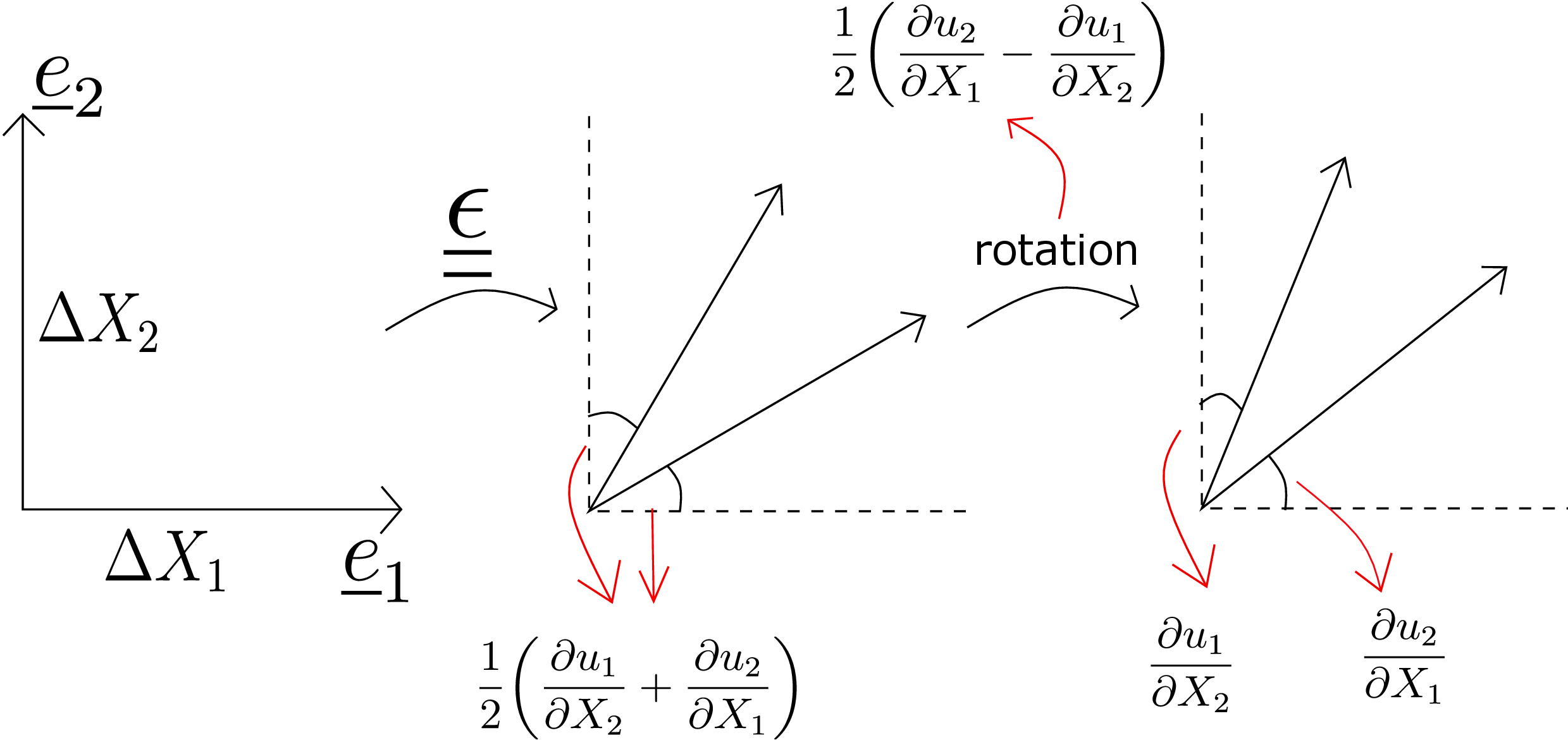
along \(\underline {e}_1\) and \(\underline {e}_2\) directions with magnitudes \(\Delta X_1\) and \(\Delta X_2\) respectively (see Figure 5.14). Let us analyze the effect of strain and rotation on their deformation separately. First, let’s consider only \(\underline {\underline {\epsilon }}\) acting on the line elements: shear strain causes change in angle between the two line elements. The total shear in this case is \begin {equation} \gamma _{12}=2\epsilon _{12}=\frac {\partial u_1}{\partial X_2}+\frac {\partial u_2}{\partial X_1} \end {equation} which can be thought of as both the line elements rotating by half of this quantity in opposite directions (see the middle of Figure 5.14). We then superimpose local rigid rotation in the second step. We can deduce the angle of local rigid rotation from equation \eqref{5_e_3_axial_vector} to be \(\dfrac {1}{2}\bigg (\dfrac {\partial u_2}{\partial X_1}-\dfrac {\partial u_1}{\partial X_2}\bigg )\). Hence, both the line elements will further rotate by this amount but in the same direction. Let us now add the rotations due to shear and rigid rotation to get total rotation of the line elements. The total rotation of line element along \(\underline {e}_1\) will be
For the line element along \(\underline {e}_2\), the rotation due to shear is in the opposite direction (clockwise). Therefore
The total rotations for the two line elements turn out to be exactly the same that we had seen earlier at the end of section 5.5 when we were discussing the geometric interpretation of shear strain formula. This also verifies that we can view the total rotation of a line element as the sum of rotations due to shear and local rigid rotation.
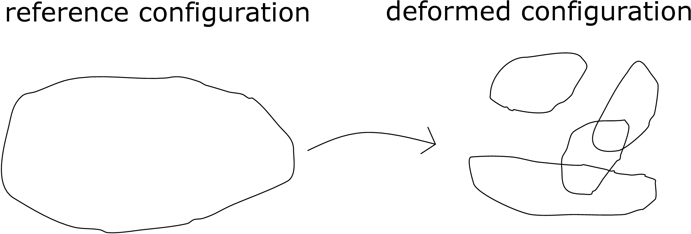
We know that the strain matrix in (\(\underline {e}_1,\underline {e}_2,\underline {e}_3\)) coordinate system is \begin {equation} \label {5_strain_in_terms_of_displacement} [\underline {\underline {\epsilon }}]=\begin {bmatrix} \frac {\partial u_X}{\partial X} & \frac {1}{2}\bigg (\frac {\partial u_X}{\partial Y}+\frac {\partial u_Y}{\partial X}\bigg ) & \frac {1}{2}\bigg (\frac {\partial u_X}{\partial Z}+\frac {\partial u_Z}{\partial X}\bigg )\\ \frac {1}{2}\bigg (\frac {\partial u_X}{\partial Y}+\frac {\partial u_Y}{\partial X}\bigg ) & \frac {\partial u_Y}{\partial Y} & \frac {1}{2}\bigg (\frac {\partial u_Y}{\partial Z}+\frac {\partial u_Z}{\partial Y}\bigg )\\ \frac {1}{2}\bigg (\frac {\partial u_X}{\partial Z}+\frac {\partial u_Z}{\partial X}\bigg ) & \frac {1}{2}\bigg (\frac {\partial u_Y}{\partial Z}+\frac {\partial u_Z}{\partial Y}\bigg ) & \frac {\partial u_Z}{\partial Z} \end {bmatrix}. \end {equation} Due to symmetry, it has only six independent components all of which are functions of (\(X,Y,Z\)) in general. Suppose, instead of obtaining strain matrix from the derivative of displacement functions, we directly write it by choosing six arbitrary functions for its components, i.e., \begin {equation} [\underline {\underline {\epsilon }}]=\begin {bmatrix} \epsilon _{xx} & \epsilon _{xy} & \epsilon _{xz}\\ \epsilon _{xy} & \epsilon _{yy} & \epsilon _{yz}\\ \epsilon _{xz} & \epsilon _{yz} & \epsilon _{zz} \end {bmatrix}. \end {equation} Will such a strain matrix correspond to any displacement function? The answer is NO! Basically, using strain-displacement relation in \eqref{5_strain_in_terms_of_displacement}, if we integrate the six arbitrary strain component functions to obtain the three displacement components, we may not obtain a consistent displacement function. For example, think of integrating \(\epsilon _{XX}(X,Y,Z)\) in \(X\) to obtain \(u_X\) and then integrating \(\epsilon _{YY}(X,Y,Z)\) in \(Y\) to obtain \(u_Y\), then the calculated \(\epsilon _{XY}\) from the so obtained \((u_X,u_Y)\) need not match with the prescribed function for \(\epsilon _{XY}\). Physically, it may also happen that the displacement so obtained is such that it leads to two parts of a body overlapping with each other or getting separated as in Figure 5.15. Thus, there has to be some constraint on the six strain functions which are collectively called strain compatibility conditions. Thus, a general symmetric matrix does not necessarily represent a strain matrix unless it satisfies these strain compatibility conditions.
Another way to look at compatibility conditions is that when we integrate a given strain matrix along an arbitrary path in the reference configuration of a body, the displacement components so obtained should just depend on the end points of the path and not on the actual path of integration. For example, suppose we start at a point A shown in Figure 5.16 and want to find the displacement of point B.
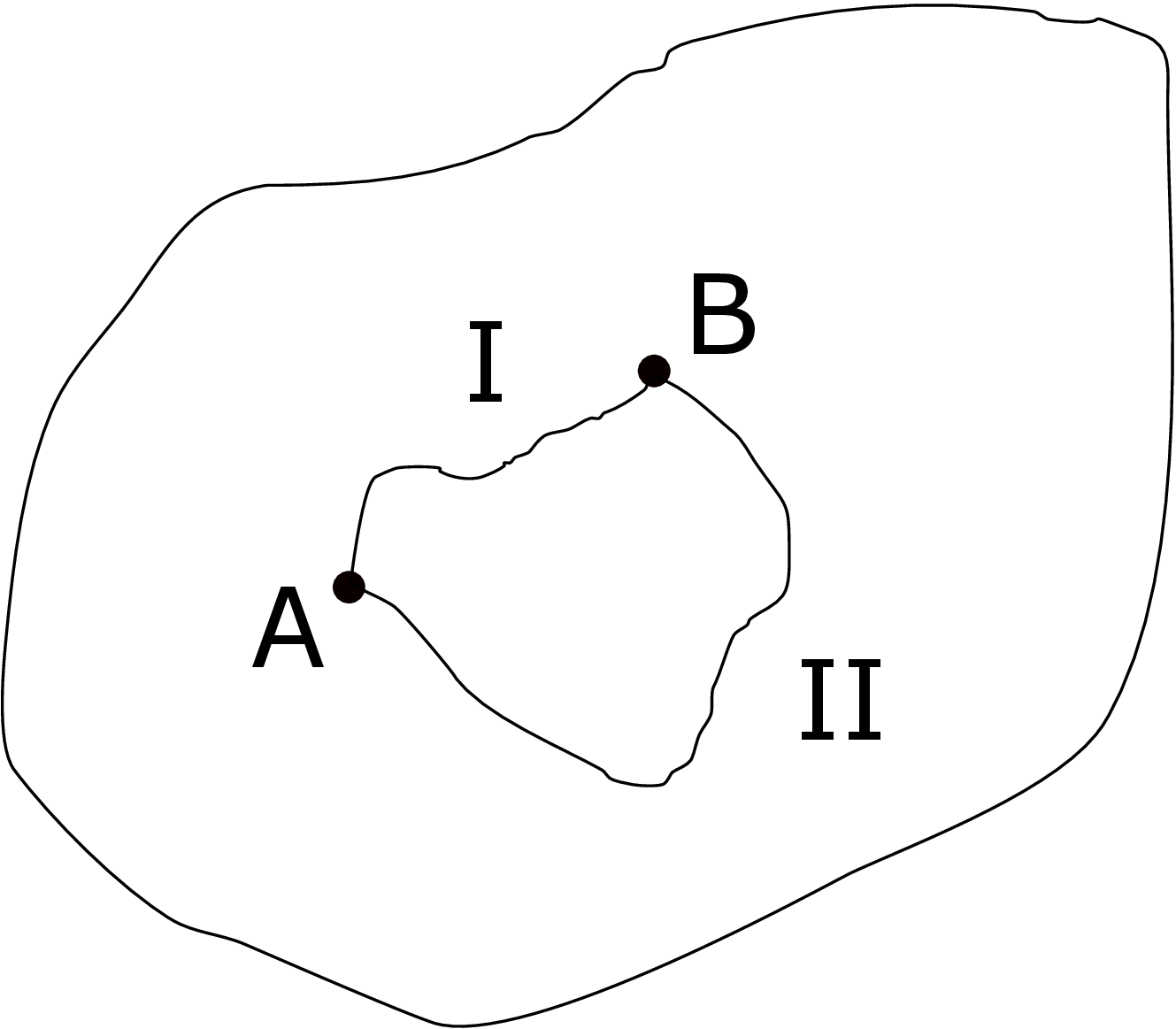
We can go through different paths and integrate the strain components along the path to find the displacement of B. Regardless of the path followed, the displacement should come out to be the same because the final point is the same and it must have a unique displacement. In other words, the integration has to be path independent and the strain compatibility conditions exactly ensure that. There is a rigorous mathematical proof to obtain strain compatibility conditions but that is out of scope of this book. There are six compatibility conditions which can be divided into two sets. The first set is
We can also verify them by plugging them into strain-displacement relation, e.g., consider the LHS of equation \eqref{5_first_condition}:
The second set of compatibility conditions is
There is a special case in which five of the compatibility conditions get satisfied automatically. Consider the following situation:
This special case is also called the plane strain condition. For such a case, it is easy to check that five of the compatibility conditions (all except equation \eqref{5_first_condition}) are automatically satisfied.
Let us list the formulas of stress and strain components derived earlier. On the stress side, we have normal (\(\sigma _{nn}\)) and shear (\(\tau _{mn}\)) components of traction while on the strain side, we have longitudinal (\(\epsilon _{nn}\)) and shear (\(\gamma _{mn}\)) strains as shown below: \begin {align*} &\textbf {Stress}\hspace {40mm}&\textbf {Strain}\\ &\sigma _{nn}=\big (\underline {\underline {\sigma }}\,\underline {n}\big )\cdot \underline {n}&\epsilon _{nn}=\big (\underline {\underline {\epsilon }}\,\underline {n}\big )\cdot \underline {n}\\ &\tau _{mn}=\big (\underline {\underline {\sigma }}\,\underline {n}\big )\cdot \underline {m}& \gamma _{mn}=2\big (\underline {\underline {\epsilon }}\,\underline {n}\big )\cdot \underline {m} \end {align*}
We can notice the similarity in above formulas. Recall, we had defined the strain tensor \(\underline {\underline {\epsilon }}\) to be \begin {equation} \underline {\underline {\epsilon }}=\frac {1}{2}\Big (\underline {\nabla }\,\underline {u}+\underline {\nabla }\,\underline {u}^T\Big ). \end {equation} Thus, the
strain tensor is also symmetric just like the stress tensor and stress and strain component formulas are also
similar. This means that we can apply all the properties derived for stress tensor to also strain tensor. Let
us now discuss them one by one.
Principal directions and principal components:
We had discussed about principal stress planes and principal stress components earlier. Likewise, we can
also define principal strain directions (not planes) and principal strain components. We know that at a
point, principal stress planes are the planes on which the normal component of traction is
maximized/minimized. The value of the normal component of traction on these planes are principal stress
components. Similarly, at a point in a body out of numerous line elements, the directions of those line
elements that experience maximum/minimum longitudinal strain are called principal strain directions. The
values of longitudinal strain in these directions are called principal strain components. To find them, we do
the same as earlier, i.e., we obtain eigenvectors and eigenvalues of the strain tensor.
Diagonality of matrix form in principal coordinate system:
We know that the stress matrix in the coordinate system of principal stress directions becomes diagonal.
Similarly, when we represent the strain matrix in the coordinate system of the principal strain directions, it
will become a diagonal matrix. As the off-diagonal components will be zero, this means that if we take two
line elements to be directed along two different principal strain directions, there will not be any change in
angle between them. To visualize this, we can consider a cuboid whose face normals are along the principal
strain directions (given by eigenvectors of the strain tensor) as shown on the left in Figure 5.17.
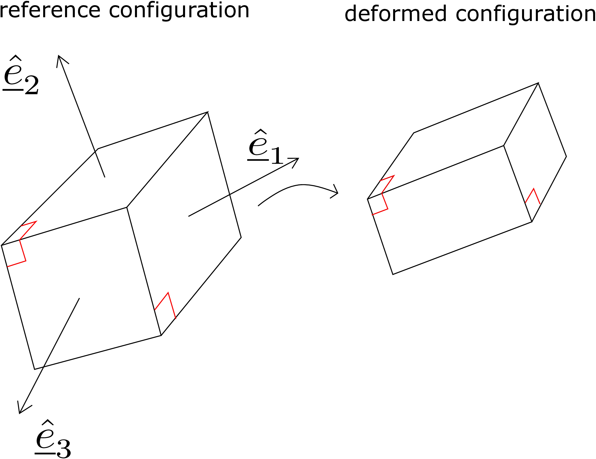
Here \(\underline {\hat e}_1,\underline {\hat e}_2, \underline {\hat e}_3\) represent principal strain directions. The cuboid gets deformed as shown on the right in Figure 5.17.
As the angle between line elements along principal directions does not change, the cuboid only changes its
size but the deformed shape is still a cuboid.
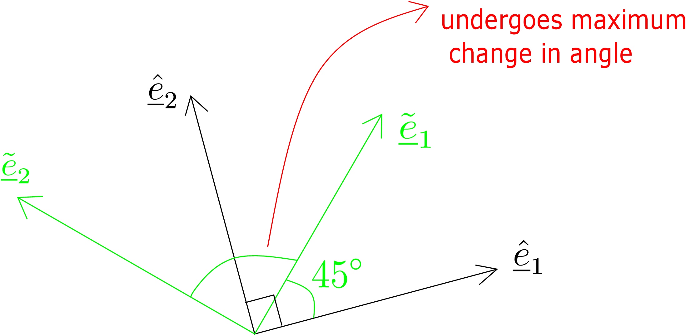
Maximum shear:
We can also maximize shear strain at a point just like we maximized the shear component of traction. We
had found that the planes on which the shear component of traction is maximized/minimized lie at an
angle of \(45^\circ \) from the principal planes. Similarly, the pair of perpendicular line elements that undergoes
maximum change in angle (or maximum shear strain) will be directed at \(45^\circ \) from principal strain directions.
This is shown in Figure 5.18.
Mohr’s circle:
We can also think of Mohr’s circle for strain. Mohr’s circle for stress gave the values of normal traction (\(\sigma \))
and shear traction (\(\tau \)) on an arbitrary plane. Similarly, if we know the value of longitudinal strain along two
perpendicular directions say \(\underline {e}_1\) and \(\underline {e}_2\) and also know shear strain between \(\underline {e}_1\) and \(\underline {e}_2\), then one can use Mohr’s circle
for strain to obtain longitudinal and shear strain for two perpendicular line elements which are oriented at
angle \(\theta \) relative to (\(\underline {e}_1\)-\(\underline {e}_2\)) pair. The strain plane will have longitudinal strain \(\epsilon \) on X-axis and half of shear strain
(\(\gamma /2\)) on Y-axis: this is because the formula for shear strain has an extra factor of 2 when compared with the
corresponding component in strain matrix. This will permit us to draw Mohr’s circle for strain in exactly
the same manner as we drew Mohr’s circle for stress. We had seen while discussing Mohr’s circle for stress
that it can be drawn only when at least one coordinate axis is along the principal stress direction. Likewise,
for Mohr’s circle for strain also, we can draw the circle only when at least one coordinate axis is along a
principal strain direction. For now, let us suppose that the third coordinate axis is along a principal strain
direction. Thus, the strain matrix in such a coordinate system will look as follows: \begin {equation} \begin {bmatrix}\underline {\underline {\epsilon }}\end {bmatrix}= \begin {bmatrix} \epsilon _{xx} & \epsilon _{xy} & 0\\ \epsilon _{xy} & \epsilon _{yy} & 0\\ 0 & 0 & \epsilon _{zz} \end {bmatrix}= \begin {bmatrix} \epsilon _{xx} & \frac {\gamma _{xy}}{2} & 0\\ \frac {\gamma _{xy}}{2} & \epsilon _{yy} & 0\\ 0 & 0 & \epsilon _{zz} \end {bmatrix} \end {equation} For drawing the Mohr’s
circle, we need to find out the center and the radius of the circle.
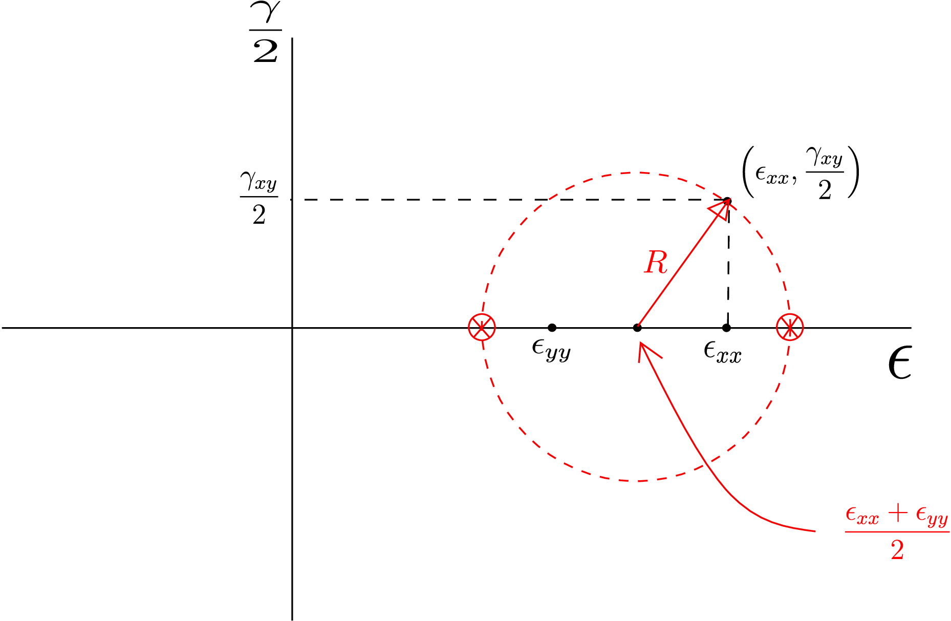
The center of the circle will be at the mid point of \(\epsilon _{xx}\) and \(\epsilon _{yy}\) on \(\epsilon \) axis. We then mark the point (\(\epsilon _{xx}\),\(\frac {\gamma _{xy}}{2}\)) as shown in Figure
5.19. Having found the center of the circle and a point on it, we get the radius by joining them as shown in Figure
5.19 which allows us to draw the full circle. The radius \(R\) can also be found by applying the Pythagoras theorem to the
right angled triangle shown there. We can extract a lot of information from this circle just like we had seen in the
stress case. For example, the principal strain components will be obtained from the points where the circle cuts the \(\epsilon \)
axis (shown in red crossed circles in Figure 5.19), i.e., \begin {equation} \text {Principal strain components: }\frac {\epsilon _{xx}+\epsilon _{yy}}{2}\pm R, \epsilon _{zz}. \end {equation} Also, maximum shear strain (\(\gamma _{max}\)) can be obtained
from the Mohr’s circle radius, i.e., \begin {equation} \gamma _{max}=2R. \end {equation} Finally, we can find longitudinal and shear strains for arbitrary
line elements. For example, to obtain longitudinal strain for a line element which makes an angle \(\theta \)
with \(\underline {e}_1\) axis in clockwise direction, we need to go anticlockwise by \(2\theta \) on the Mohr’s circle from (\(\epsilon _{xx}\),\(\frac {\gamma _{xy}}{2}\)). For
getting shear strain, remember that we need to multiply the value obtained from the Mohr’s circle by
2.
Invariants:
Just like we have invariants of the stress tensor as \(I_1\), \(I_2\) and \(I_3\), we also have invariants of the strain tensor denoted by \(J_1\), \(J_2\)
and \(J_3\). They are exactly analogous to each other, e.g., \(J_1\) represents the trace of strain tensor (just like \(I_1\) represents the
trace of stress tensor).
Decomposition of strain tensor:
We had learnt about the decomposition of stress tensor into hydrostatic and deviatoric parts. We can also decompose
the strain tensor into two parts in a similar way as shown below: \begin {equation} \underline {\underline {\epsilon }}=\underbrace {\frac {1}{3}J_1~\underline {\underline {I}}}_{\text {volumetric strain tensor}}+\underbrace {\bigg (\underline {\underline {\epsilon }}-\frac {1}{3}J_1~\underline {\underline {I}}\bigg )}_{\text {strain deviator}} \end {equation} The first part is proportional to identity. It is
analogous to the hydrostatic part of stress and is called the volumetric strain tensor. This part is responsible for
change in volume and does not affect the shape of the body. The second part is analogous to the stress deviator
and is called the strain deviator. Its trace is zero by construction and is responsible for distorting the
body.
Q1. Think of the following displacement field: \begin {align*} u_1 &= 0.05 x_1 + 0.03 x_2^2,\\ u_2 &= 0.07 x_1 x_2 + 0.08 x_1^2,\\ u_3 &= 0. \end {align*}
Solution: \begin {align*} \sbk {\ve {\nabla } \; \ve {u}} = \begin {bmatrix} \dfrac {\partial u_1}{\partial x_1} & \dfrac {\partial u_1}{\partial x_2} & \dfrac {\partial u_1}{\partial x_3}\\ \dfrac {\partial u_2}{\partial x_1} & \dfrac {\partial u_2}{\partial x_2} & \dfrac {\partial u_2}{\partial x_3}\\ \dfrac {\partial u_3}{\partial x_1} & \dfrac {\partial u_3}{\partial x_2} & \dfrac {\partial u_3}{\partial x_3} \end {bmatrix} = \begin {bmatrix} 0.05 & 0.06x_2 & 0 \\ 0.07x_2\;+\;0.16x_1 & 0.07x_1 & 0\\ 0 & 0 & 0 \end {bmatrix}. \end {align*}
Therefore \begin {align*} \sbk {\ve {w}}\;=\;\begin {bmatrix} 0\\ 0\\ -\dfrac {1}{2}\brc {\dfrac {\partial u_1}{\partial x_2}\;-\;\dfrac {\partial u_2}{\partial x_1}} \end {bmatrix}=\;\begin {bmatrix} 0\\ 0\\ 0.005x_2\;+0.08x_1 \end {bmatrix}. \end {align*}
For an exhaustive set of solved examples and unsolved objective and subjective type questions, please refer to the printed book.
∗In the first example, the change in length for every line element turns out to be the same, so the local strain at any point in the bar equals the global strain.
†Line elements can be thought of as the collection of material points of the body along the line drawn in it.
‡We had already discussed ‘o(\(\cdot \))’ notation (pronounced small-oh) which meant that the terms are of higher order. So, we could also categorize O(\(\vert \vert \Delta \underline {X}\vert \vert ^2\)) terms as o(\(\vert \vert \Delta \underline {X}\vert \vert \)) terms.
§Remember that an \(O(\vert \vert \Delta \underline {X}\vert \vert ^n)\) term also contains \(O(\vert \vert \Delta \underline {X}\vert \vert ^{n+1})\), \(O(\vert \vert \Delta \underline {X}\vert \vert ^{n+2})\) and all further higher order terms: sum of all these can be written together as \(O(\vert \vert \Delta \underline {X}\vert \vert ^n)\).
¶It is a good practice to keep such terms till the end and not neglect them in the beginning itself. If we discard any term right in the beginning, we would never come to know if that could have become a significant term later.
ʺAs we had discussed earlier, for small enough initial line elements, the deformed line elements can also be approximated as straight lines.
∗∗A square matrix when added to its transpose will always result in a symmetric matrix.
††The trace of a square matrix is equal to the sum of the diagonal elements of the matrix.