By now we have learnt that at any point in a body, we have different traction vector on different planes. Among these planes, the planes on which the normal component of traction becomes maximum are called principal planes and the corresponding values of the normal traction component are called principal stress components. The knowledge of such planes is of significant importance because according to one of the failure theories, a body fails at a point if the largest principal stress component there reaches a threshold limit. For the same reason, it is also of importance to know the planes on which the shear component of traction becomes maximum. In this chapter, we will derive formulas for such plane normals. Later on, we will talk about Mohr’s circle - a graphical technique to find normal and shear components of traction on arbitrary planes at a point. Finally, we will talk about the concept of stress invariants, octahedral stress component and the decomposition of stress tensor.
Let us now try to find formulas for principal planes. The normal component of traction on an arbitrary plane with normal \(\underline {n}\) is given by \begin {equation} \sigma _{nn}=\underline {t}^n\cdot \underline {n}=(\underline {\underline {\sigma }}\,\underline {n})\cdot \underline {n}. \end {equation} Our objective is to maximize it. We know from the first year calculus that once we have a mathematical formula for a quantity (in terms of unknown variables) to be maximized/minimized, we set the derivative of the quantity with respect to all variables to zero and solve the resulting equations to obtain the unknown variables. Let us choose a coordinate system (\(\underline {e}_1, \underline {e}_2, \underline {e}_3\)) and write the formula for \(\sigma _{nn}\) in this coordinate system, i.e.,
The normal direction (or the three components (\(n_1, n_2,n_3\))) is an unknown here while the stress matrix would be known/prescribed. However, the normal vector being of unit magnitude, its three components must satisfy \begin {equation} \label {4_magnitude_unity} {n}_1^2+{n}_2^2+{n}_3^2-1=0. \end {equation} This implies that the three components are not all independent, e.g., \(n_3\) can be written in terms of the other two as follows: \begin {equation} {n}_3=\sqrt {1-{n}_1^2-{n}_2^2}. \end {equation} We can substitute the above formula for \(n_3\) in equation \eqref{4_normal_component_equation} and then differentiate the resulting expression for \(\sigma _{nn}\) just with respect to \({n}_1\) and \({n}_2\). However, the modified expression for \(\sigma _{nn}\) would become a bit complex differentiating which and further solving the resulting equations would not be easy. Another way to maximize/minimize the function \eqref{4_normal_component_equation} in presence of constraint \eqref{4_magnitude_unity} is the method of Lagrange multipliers which we now discuss.
In this method, the objective function (the function to be minimized/maximized) is augmented by adding or subtracting to it the constraint equation multiplied with an unknown Lagrange multiplier. So, the augmented function (denoted by \(f\)) now becomes a function of the three components (\({n}_1\), \({n}_2\), \({n}_3\)) and the Lagrange multiplier \(\lambda \) as follows: \begin {equation} f(n_1,n_2,n_3,\lambda )=\sum _{i}\sum _{j}\sigma _{ij}n_j n_i-\lambda \Big (\sum _{i}n_i n_i-1\Big ). \end {equation} The term \(\Big (\sum _{i}n_i n_i-1\Big )\) is our constraint equation \eqref{4_magnitude_unity} and the negative sign in front of it could also have been a positive sign. This sign does not make any difference to the overall formulation and the final result. We then take the derivative of \(f\) with respect to each of the unknowns, i.e., (\({n}_1\),\({n}_2\),\({n}_3\),\(\lambda \)). Let us begin by taking the derivative with respect to \({n}_1\): \begin {equation} \label {4_derivative_n1} \frac {\partial f}{\partial n_1}=\sum _{i}\sum _{j}\sigma _{ij} \frac {\partial n_j}{\partial n_1}n_i +\sum _{i}\sum _{j} \sigma _{ij}n_j\frac {\partial n_i}{\partial n_1}-\lambda \Big (\sum _{i} 2 \frac {\partial n_i}{\partial n_1}n_i\Big ). \end {equation} As \(\sigma _{ij}\) is a constant here, it does not get differentiated. Furthermore, as \({n}_1\), \({n}_2\) and \({n}_3\) can be taken to be independent now∗, we can write
The derivative expression in \eqref{4_derivative_n1} can be generalized by taking the derivative of \(f\) with respect to a general component \(n_k\) as shown below: \begin {equation} \frac {\partial f}{\partial n_k}=\sum _{i} \sum _{j} \sigma _{ij} \delta _{jk} n_i +\sum _{i} \sum _{j} \sigma _{ij} n_j \delta _{ik} -2\lambda \sum _{i}\delta _{ik}n_i=0. \end {equation} Using the Kronecker delta property, it further simplifies to \begin {equation} \sum _{i} \sigma _{ik} n_i+\sum _{j} \sigma _{kj} n_j -2 \lambda ~ n_k=0. \end {equation} The first two terms here can be clubbed together because \(i\) and \(j\) are just dummy variables (variable of summation) which can be replaced with any other variable. Thus \begin {equation} \sum _{i}(\sigma _{ik}+\sigma _{ki})n_i -2 \lambda n_k=0. \end {equation} Finally, as the stress matrix is symmetric, we get \begin {equation} \label {4_derivative_nk} \boxed {\sum _{i}\sigma _{ki}n_i=\lambda n_k ~\text {for}~k=1,2,3} \end {equation} We now take the derivative of \(f\) with respect to \(\lambda \), i.e., \begin {equation} \label {4_derivative_lambda} \frac {\partial f}{\partial \lambda }=\sum _{i} n_i n_i-1=0. \end {equation} So, we have four equations in total (three from equation \eqref{4_derivative_nk} and one from equation \eqref{4_derivative_lambda}) for the four unknowns (\(n_1,n_2,n_3,\lambda \)). Equation \eqref{4_derivative_nk} can be written in a matrix form since for each k, the first term on the LHS of \eqref{4_derivative_nk} can be obtained by multiplying the \(k^{th}\) row of \(\begin {bmatrix} \underline {\underline {\sigma }} \end {bmatrix}\) with the column of \(\underline {n}\). This leads to \begin {equation} \label {4_matrixform_eigen} \begin {bmatrix} \underline {\underline {\sigma }} \end {bmatrix} \begin {bmatrix} \underline {n} \end {bmatrix}=\lambda \begin {bmatrix} \underline {n} \end {bmatrix}. \end {equation} We immediately see that this is an eigenvalue-eigenvector problem. We also know from first year mathematics that if \(\underline {x}\) is an eigenvector, then a scalar multiple of \(\underline {x}\) is also an eigenvector which can be proved as follows:
Thus both \(\underline {x}\) and \(b\underline {x}\) are eigenvectors having the same eigenvalue \(\lambda \) for an arbitrary scalar \(b\). Thus, the magnitude of our direction vector \(\underline {n}\) could be anything as far as equation \eqref{4_matrixform_eigen} is concerned but equation \eqref{4_derivative_lambda} restricts its magnitude to be unity. Also when we relook at equation \eqref{4_matrixform_eigen}, the left hand side is nothing but the column representation of traction on a plane with normal \(\underline {n}\). Thus, we have \begin {equation} \label {traction_principal_planes} \underline {t}^n=\underline {\underline {\sigma }}\,\underline {n}=\lambda ~\underline {n}\nonumber \\ \Rightarrow \sigma _{nn} = \underline {t}^n\cdot \underline {n}=\lambda ~\underline {n}\cdot \underline {n}=\lambda . \end {equation} From this, we immediately infer that the traction on a plane with normal \(\underline {n}\) (given by \eqref{4_matrixform_eigen}) acts along the direction \(\underline {n}\) itself and hence has no shear component. Summarizing, the principal planes of stress at a point have their normals equal to eigenvectors of the stress tensor whereas the principal stress components are given by eigenvalues of the stress tensor.
By definition, principal planes are the planes on which the normal component of traction is maximized/minimized. Their normals turn out to be the eigenvectors of the stress tensor. We want to know how many such planes exist at any given point in the body. As stress matrix is a \(3\times 3\) matrix, it will usually have three eigenvalues and eigenvectors but they need not all be real. However, being symmetric ensures that these eigenvalues and eigenvectors are all real. In fact, for symmetric matrices, the eigenvectors corresponding to distinct eigenvalues are perpendicular to each other too. To prove this, consider two eigenvectors \(\underline {n}_1\) and \(\underline {n}_2\) of a symmetric tensor \(\underline {\underline {\sigma }}\) with corresponding eigenvalues \(\lambda _1\) and \(\lambda _2\) (but distinct). Thus, we have
Let us take the dot product of first equation with \(\underline {n}_2\) and of the second equation with \(\underline {n}_1\). This yields
We consider equation \eqref{4_ortho_2} now where we take \(\underline {\underline {\sigma }}\) to the other side of the dot product by taking its transpose, i.e.,
However, the stress tensor being symmetric, we get \begin {equation} \label {4_ortho_2final} (\underline {\underline {\sigma }}\,\underline {n}_1)\cdot \underline {n}_2=\lambda _2(\underline {n}_2\cdot \underline {n}_1). \end {equation} Now, we subtract equation \eqref{4_ortho_2final} from equation \eqref{4_ortho_1} which yields
As \(\lambda _1\) and \(\lambda _2\) are distinct, \(\underline {n_1}\cdot \underline {n_2}\) has to be zero implying that the two eigenvectors are perpendicular to each other. It is also easy to show that if two of the eigenvalues turn out to be the same, then any linear combination of the two eigenvectors is also an eigenvector. For example,
Summing the above two equations, we get \begin {equation} \underline {\underline {\sigma }}\,(\alpha \underline {n}_1+\beta \underline {n}_2)=\lambda ~ (\alpha \underline {n}_1+\beta \underline {n}_2). \end {equation} This implies that if two of the eigenvalues repeat, there exists infinite number of eigenvectors formed by arbitrary linear combination of \(\underline {n}_1\) and \(\underline {n}_2\) all of which by definition are also the principal planes and having the same eigenvalue or principal stress component. Among these infinite possibilities, we can always choose two which are perpendicular to each other. Thus, we can always pick a set of three orthonormal eigenvectors or three orthonormal principal planes at a point.
Let us choose the three perpendicular eigenvectors to be the basis vectors of a coordinate system and represent the stress tensor in this coordinate system. As per definition, we first find traction on planes having normals along the basis vectors. As the basis vectors are themselves the eigenvectors of stress tensor, traction on those planes will simply be \(\lambda \underline {n}\) (no shear component present). Thus, the corresponding stress matrix will become a diagonal matrix as shown below: \begin {equation} \begin {bmatrix} \underline {\underline {\sigma }} \end {bmatrix}= \begin {bmatrix} \lambda _1 & 0 & 0\\ 0 & \lambda _2 & 0\\ 0 & 0 & \lambda _3 \end {bmatrix}. \end {equation}
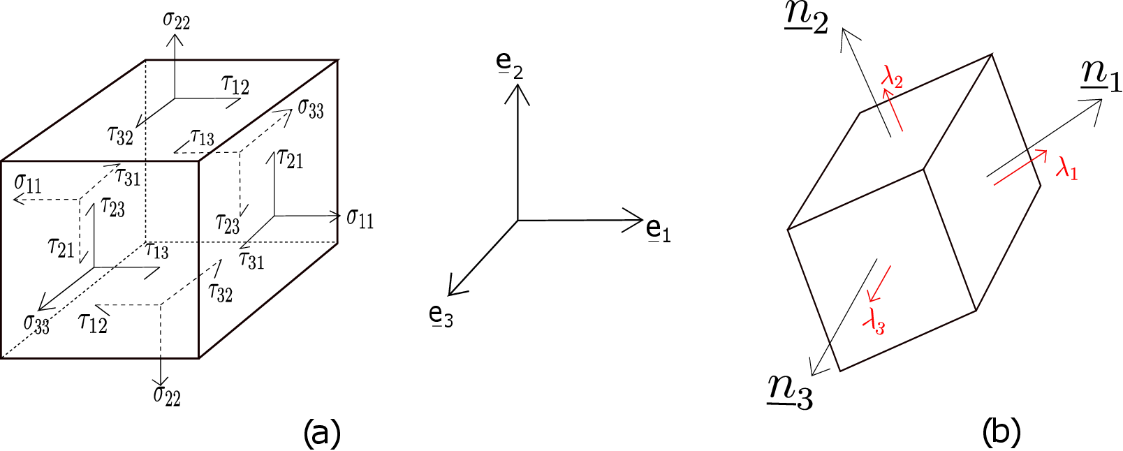
Alternatively, given an arbitrary stress matrix in some coordinate system, we can always transform it to become diagonal in the coordinate system whose basis vectors are aligned with the eigenvectors of the stress tensor. In the general case as shown in Figure 4.1a, both normal and shear components of traction are present on the faces of a cuboid element at a point in the body. However, if we choose the cuboid element in such a way that its faces are the principal planes as shown in Figure 4.1b, its faces will then have no shear component and only normal components (\(\lambda _1\), \(\lambda _2\), \(\lambda _3\)) will be present. So, the faces of this cuboid will have no tendency to shear. The opposite faces can only get either pulled apart or pushed inside depending on the sign of \(\lambda \).
To obtain the maxima or minima of shear component of traction at a point, we need to first find its expression on an arbitrary plane. Let us consider a part of the body as shown in Figure 4.2.
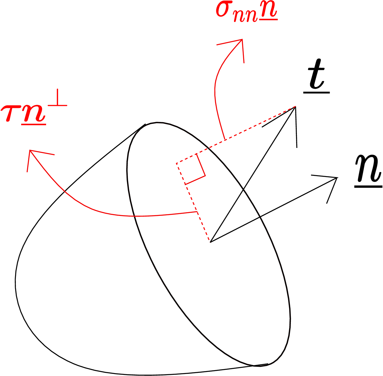
The plane shown has normal \(\underline {n}\) and the traction on it is denoted by \(\underline {t}\). Earlier, we had noted that the normal component of traction is given by \begin {equation} \label {traction_normal} \sigma _{nn}=\underline {t}\cdot \underline {n}. \end {equation} To obtain the shear component of traction, we can subtract this normal component from the total traction vectorially. In Figure 4.2 for example, the traction \(\underline {t}\) has been decomposed into normal and shear components. The projection of traction along \(\underline {n}\) is the normal component given by \(\sigma _{nn}~\underline {n}\) while the remaining component (perpendicular to \(\underline {n}\)) is the shear part denoted by \(\tau \underline {n}^\perp \). Here \(\tau \) denotes magnitude and \(\underline {n}^{\perp }\) the direction (perpendicular to \(\underline {n}\)) along which the shear part of traction acts. Applying Pythagoras theorem to the right-angled triangle formed by traction and its components as shown in Figure 4.2, we can write†
This formula when expressed in a coordinate system will become lengthy. However, in the coordinate system of principal directions, the stress matrix will be a diagonal matrix which will simplify the above formula as shown below:
Keep in mind that that this is the magnitude square of total/resultant shear that acts along a direction given by the vector sum of two shear components on a plane. For example, on \(\underline {e}_1\) plane, we have both \(\tau _{21}\) and \(\tau _{31}\). The vector resultant of these two components gives us the square of magnitude of total shear to be \(\tau _{21}^2+\tau _{31}^2\) - we will obtain the same from equation \eqref{4_shear_magnitude_principal}.
In formula \eqref{4_shear_magnitude_principal}, \({n}_1\), \({n}_2\) and \({n}_3\) are unknowns but they are not independent of each other. We therefore again use the method of Lagrange multiplier and define a function \(V\) as shown below: \begin {equation} V=\sum _{i} \lambda _i^2 n_i^2-\Big (\sum _{i} \lambda _i n_i^2 \Big )^2+\alpha \Big (\sum _{i} n_i n_i-1\Big ). \end {equation} Here \(\alpha \) is the Lagrange multiplier. The above function has to be maximized with respect to the 4 unknowns: \(n _1\), \(n _2\), \(n _3\) and \(\alpha \). Let us take the derivative of \(V\) with respect to these four unknowns starting with the \(k^{th}\) component of normal vector (\(n_k\)):
We have three equations here for every component of normal, i.e., \(k=1,2,3\). The fourth equation is obtained by taking the derivative with respect to \(\alpha \) and equating to zero which yields \(\sum _{i} n_i n_i-1=0.\) This is our constraint itself (i.e., magnitude of \(\underline {n}\) has to be unity). Let us write equation \eqref{4_delV_delnk} for each \(k\) separately, i.e.,
In each of these equations, one among the two terms multiplied has to be zero for the product to be zero. Therefore, there are multiple solutions to this problem. For example, choose \(n_1=0\) from the first equation, \(n_2=0\) from the second and \(n_3=0\) from the third - we get a trivial solution for \(n_1\), \(n_2\) and \(n_3\) but that will not give us a valid direction as the magnitude of the direction vector will not be 1. So, let us instead set the second term to be zero in the last two equations above.‡ So, we have the following equations at hand now:
Equations \eqref{4_second_part_2} and \eqref{4_second_part_3} have been obtained after substituting \(n_1=0\) in them. We need to find \(n_2\) and \(n_3\) now. To eliminate \(\alpha \), we subtract \eqref{4_second_part_3} from \eqref{4_second_part_2} which yields
As \(\lambda _2\) and \(\lambda _3\) are principal stress components, they are fixed at a given point in space and do not depend on what plane we are considering. Also, as this analysis holds for an arbitrary stress matrix at a point of interest, \(\lambda _2\) and \(\lambda _3\) can be assumed to be arbitrary. Thus, equation \eqref{4_arbitrary_lambda} should hold for all \(\lambda _2\) and \(\lambda _3\) implying that the coefficients of \(\lambda _2\) and \(\lambda _3\) must vanish independently. This leads to the following first set of four solutions: \begin {equation} \label {4_solution1} n_1=0,\quad n_2=\pm \frac {1}{\sqrt {2}},\quad n_3=\pm \frac {1}{\sqrt {2}}. \end {equation} But these are not the only solutions. If we had set either \(n_2\)=0 or \(n_3=0\) instead of \(n_1=0\) in the system of equations \eqref{4_eitherzero_1}, \eqref{4_eitherzero_2} and \eqref{4_eitherzero_3}, a similar analysis as above would have yielded the remaining two sets of four solutions each, i.e.,
So, we have 12 solutions in total given by equations \eqref{4_solution1}, \eqref{4_solution2} and \eqref{4_solution3}. Keep a note that these directions are with respect to the coordinate system of principal planes. For example, if we choose the solution \(n_1=\frac {1}{\sqrt {2}}\), \(n_2=\frac {1}{\sqrt {2}}\), \(n_3=0\), this tells us that the direction \(\underline {n}\) has to be perpendicular to the third principal plane’s normal. At the same time, it also makes equal angle of \(45 ^{\circ }\) with the first and second principal axes. If we look at all the 12 solutions, at least one component of \(\underline {n}\) is zero. So, each of these directions are perpendicular to at least one of the principal axes. The first set \eqref{4_solution1} is perpendicular to the first principal axis, the second set \eqref{4_solution2} is perpendicular to the second principal axis and the third set \eqref{4_solution3} is perpendicular to the third principal axis.
Let us first obtain the value of shear component of traction on these planes. We just need to plug in the solution for \(\underline {n}\) into equation \eqref{4_shear_magnitude_principal}. For the set of solutions given by equation \eqref{4_solution3}, we get
Therefore, the maximum value of shear traction is half of the difference of principal stress components. The value of the normal component of traction on this plane will be obtained by substituting \eqref{4_solution3} in expression of \(\sigma _{nn}\), i.e.,
Similarly, for the solution set \eqref{4_solution1}, we get \begin {equation} \vert \tau _{max}\vert =\Bigg \vert \frac {\lambda _2-\lambda _3}{2}\Bigg \vert ,\quad \sigma _{nn}=\frac {\lambda _2+\lambda _3}{2} \end {equation} and for the solution set \eqref{4_solution2}, we get \begin {equation} \vert \tau _{max}\vert =\Bigg \vert \frac {\lambda _1-\lambda _3}{2}\Bigg \vert ,\quad \sigma _{nn}=\frac {\lambda _1+\lambda _3}{2}. \end {equation} To visualize these results, we draw a cuboid at the point of interest with their faces being principal planes as shown in black in Figure 4.3a.
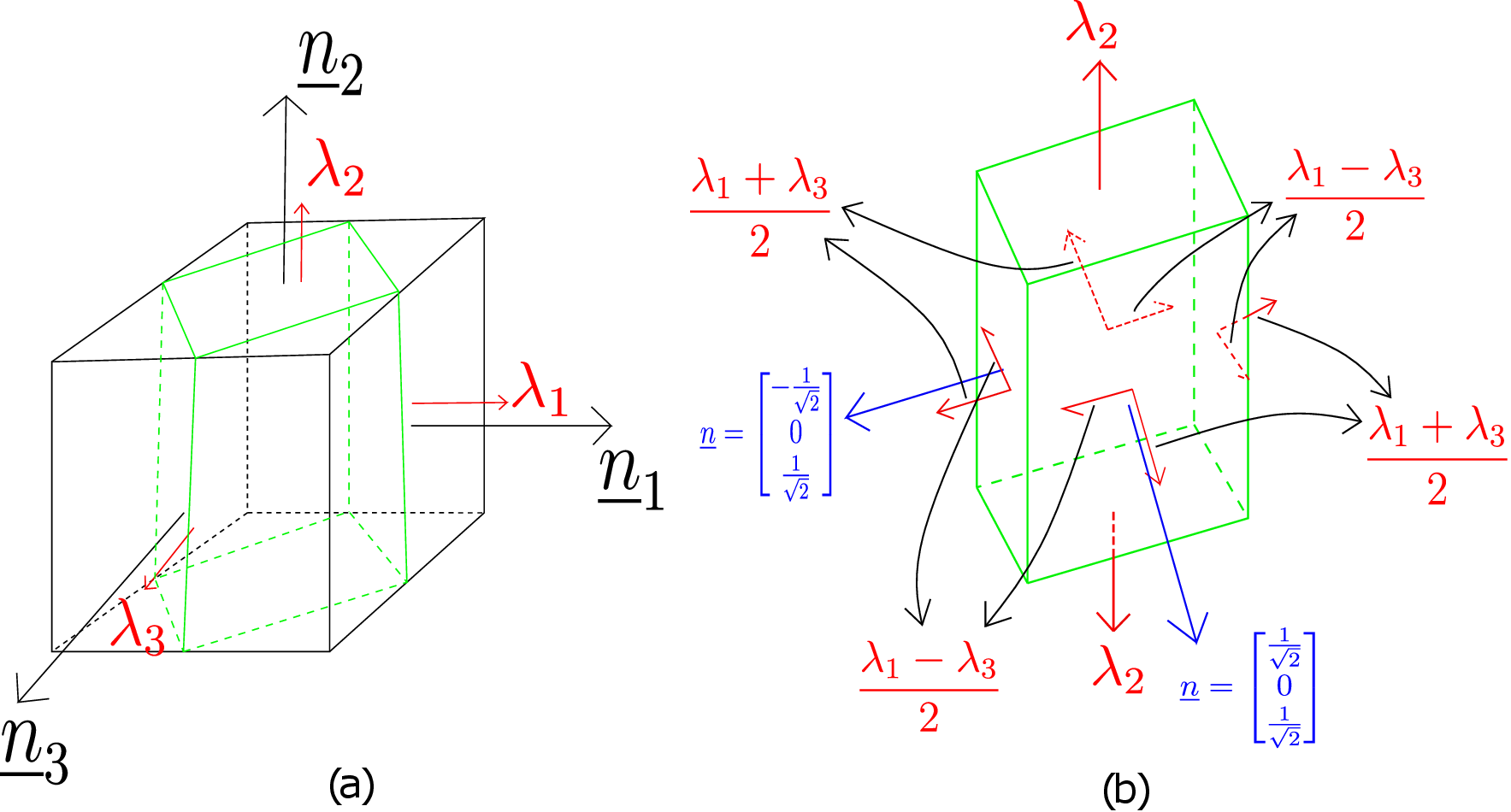
Accordingly, these faces only have normal component of traction. We want to now draw the planes corresponding to maximum shear. Let us consider the solution set where the second normal component \(n_2=0\), i.e., given by \eqref{4_solution2}. The corresponding planes are drawn in green in Figure 4.3a. We now extract this green cuboid out and look at it in isolation as shown in Figure 4.3b. On the front face of this cuboid, the normal is such that it makes equal angle with the first and third principal axes and is perpendicular to the second principal axis. For the leftmost plane, its normal’s first component is negative and the third component is positive but both having magnitude \(\frac {1}{\sqrt {2}}\). We also know the normal and shear components of traction on these planes. For example, on the front face, the normal component is \(\dfrac {\lambda _1+\lambda _3}{2}\) wheres the shear component is \(\Bigg \vert \dfrac {\lambda _1-\lambda _3}{2}\Bigg \vert \). The top face of this green cuboid has only normal component \(\lambda _2\) as it is a principal plane. We can observe that all the four planes having maximum shear component of traction are at \(45 ^{\circ }\) relative to two of the principal axes. To end the discussion, note that when we were maximizing the normal component of traction, shear component of traction on those planes turned out to be zero. But here, when we maximize the shear component of traction, the normal component of traction on these planes are not zero.
Mohr’s circle is a graphical way to find normal and shear components of traction on arbitrary planes. The only restriction is that the normal to those planes must be perpendicular to one of the principal directions. Accordingly, let us consider a coordinate system such that its third coordinate axis is along one of the principal directions. The stress matrix in this coordinate system will be such that its third column will have no shear component. The symmetry of stress matrix further forces it to have the following form: \begin {equation} \label {4_stress_representation} \begin {bmatrix} \underline {\underline {\sigma }} \end {bmatrix} =\begin {bmatrix} \times & \times &0\\ \times & \times &0\\ 0 & 0 &\times \end {bmatrix}. \end {equation}
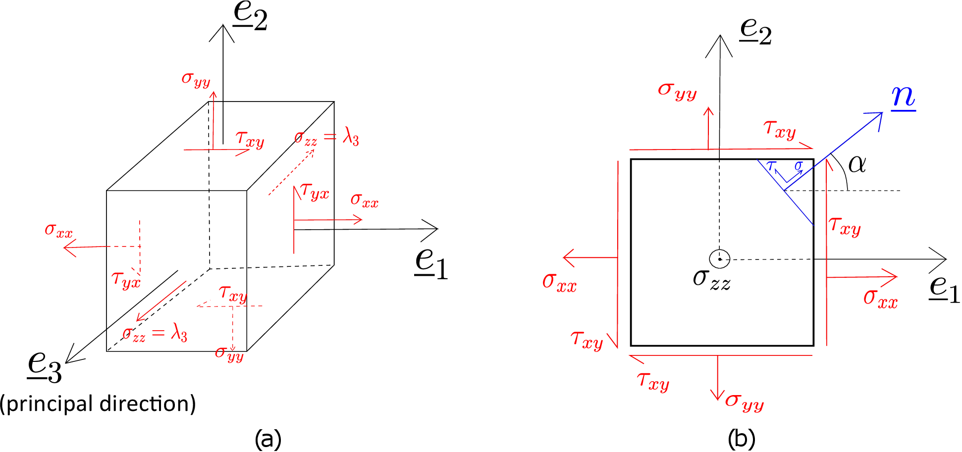
Let us draw a cuboid element at the point of interest having its faces aligned with the above mentioned coordinate system (see Figure 4.4a). We will call \(\underline {e}_1\), \(\underline {e}_2\) and \(\underline {e}_3\) axes as \(x\), \(y\) and \(z\) axes, respectively. On \(x\)-face there, we have normal component of traction shown as \(\sigma _{xx}\) and shear component of traction shown as \(\tau _{yx}\) pointing along \(y\) axis. The third component (\(\tau _{zx}\)) is absent as per the stress representation \eqref{4_stress_representation}. On \(y\)-face, we similarly have \(\sigma _{yy}\) and \(\tau _{xy}\) (same as \(\tau _{yx}\)) and on \(z\)-face, we have only \(\sigma _{zz}\) (equal to \(\lambda _3\)). There is a simpler way to draw such a state of stress: we can just draw a square instead of a cube where the sides of the square denote the faces of the cuboid as shown in Figure 4.4b. The right edge of the square represents the cuboid’s \(x\)-face, the top edge of the square represents the cuboid’s \(y\)-face and likewise. The plane of the square itself represents the cuboid’s \(z\)-face. So, the plane of the square has just one traction component \(\sigma _{zz}\) for which we use a dot enclosed by a circle. On the edges of the square, we have both normal and shear components of traction.
Our goal is to calculate the normal and shear components of traction on planes whose normals are perpendicular to \(\underline {e}_3\). The blue line in Figure 4.4b shows a general plane of such kind. Let us assume that its normal (denoted by \(\underline {n}\)) makes an angle \(\alpha \) with \(x\)-axis. The column representation of \(\underline {n}\) in (\(\underline {e}_1,\underline {e}_2,\underline {e}_3\)) coordinate system will therefore be \begin {equation} \label {n} \begin {bmatrix} \underline {n} \end {bmatrix}= \begin {bmatrix} cos(\alpha )\\ sin(\alpha )\\ 0 \end {bmatrix}. \end {equation} The normal component \(\sigma \) on this plane will be given by
To obtain the shear component \(\tau \), we first note that we have assumed that the direction of \(\tau \) on this plane makes \(90 ^{\circ }\) (anti-clockwise) from the normal vector \(\underline {n}\) (see Figure 4.4b). Accordingly, the shear direction \(\underline {n}^\perp \) is given by \begin {equation} \label {n_perp} \underline {n}^\perp = \begin {bmatrix} -sin(\alpha )\\ ~cos(\alpha )\\ 0 \end {bmatrix} \end {equation} while the shear traction \(\tau \) is given by
Upon doing some algebraic manipulation in equation \eqref{4_sigma}, we can rewrite it as follows: \begin {equation} \sigma =\frac {\sigma _{xx}+\sigma _{yy}}{2}+\sigma _{xx}\bigg (cos^2(\alpha )-\frac {1}{2}\bigg )+\sigma _{yy}\bigg (sin^2(\alpha )-\frac {1}{2}\bigg )+2\tau _{xy}sin(\alpha )cos(\alpha ). \end {equation} Further, using the following trigonometric identities:
we obtain
Similar rearrangements and simplifications using trigonometric identities \eqref{4_trigo1} and \eqref{4_trigo2} in equation \eqref{4_tau}, we get \begin {equation} \label {4_simplified_tau} \tau =-\bigg (\frac {\sigma _{xx}-\sigma _{yy}}{2}\bigg )sin(2 \alpha )+\tau _{xy}cos(2 \alpha ). \end {equation} Let us now define a scalar \(R\) as follows: \begin {equation} \label {4_R} R=\sqrt {\bigg (\frac {\sigma _{xx}-\sigma _{yy}}{2}\bigg )^2+\tau ^2_{xy}}. \end {equation} We can then think of a right angled triangle having hypotenuse \(R\) and its two perpendicular arms being \(\dfrac {\sigma _{xx}-\sigma _{yy}}{2}\) and \(\tau _{xy}\) as shown in Figure 4.5.
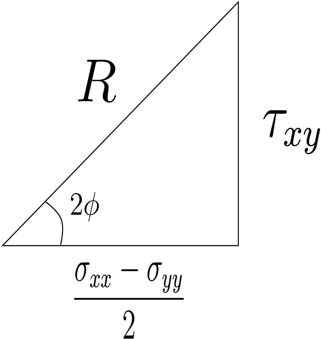
Let us also assume the angle between the hypotenuse and the base to be \(2\phi \). Thus, from basic trigonometry, we see that
Using equation \eqref{4_phi_equations} in equations \eqref{4_simplified_sigma} and \eqref{4_simplified_tau}, we then get
Upon further using the following trigonometric identities:
we finally obtain \begin {equation} \label {4_final_components} \boxed { \begin {array}{rcl} \sigma &=&\dfrac {\sigma _{xx}+\sigma _{yy}}{2}+R cos(2 \phi -2\alpha )\\\\ \tau &=&R sin(2\phi - 2\alpha ) \end {array} } \end {equation} These are the formulas for getting \(\sigma \) and \(\tau \) on a plane whose normal makes an angle \(\alpha \) with \(\underline {e}_1\) axis. Let us try to obtain the locus of the two formulas in the above box for all \(\alpha \) values.
Let us think of a \(\sigma -\tau \) plane and plot \(\sigma \) and \(\tau \) for each \(\alpha \) value in this plane. The plane with \(\sigma \) on x-axis and \(\tau \) on y-axis is shown in Figure 4.6a.
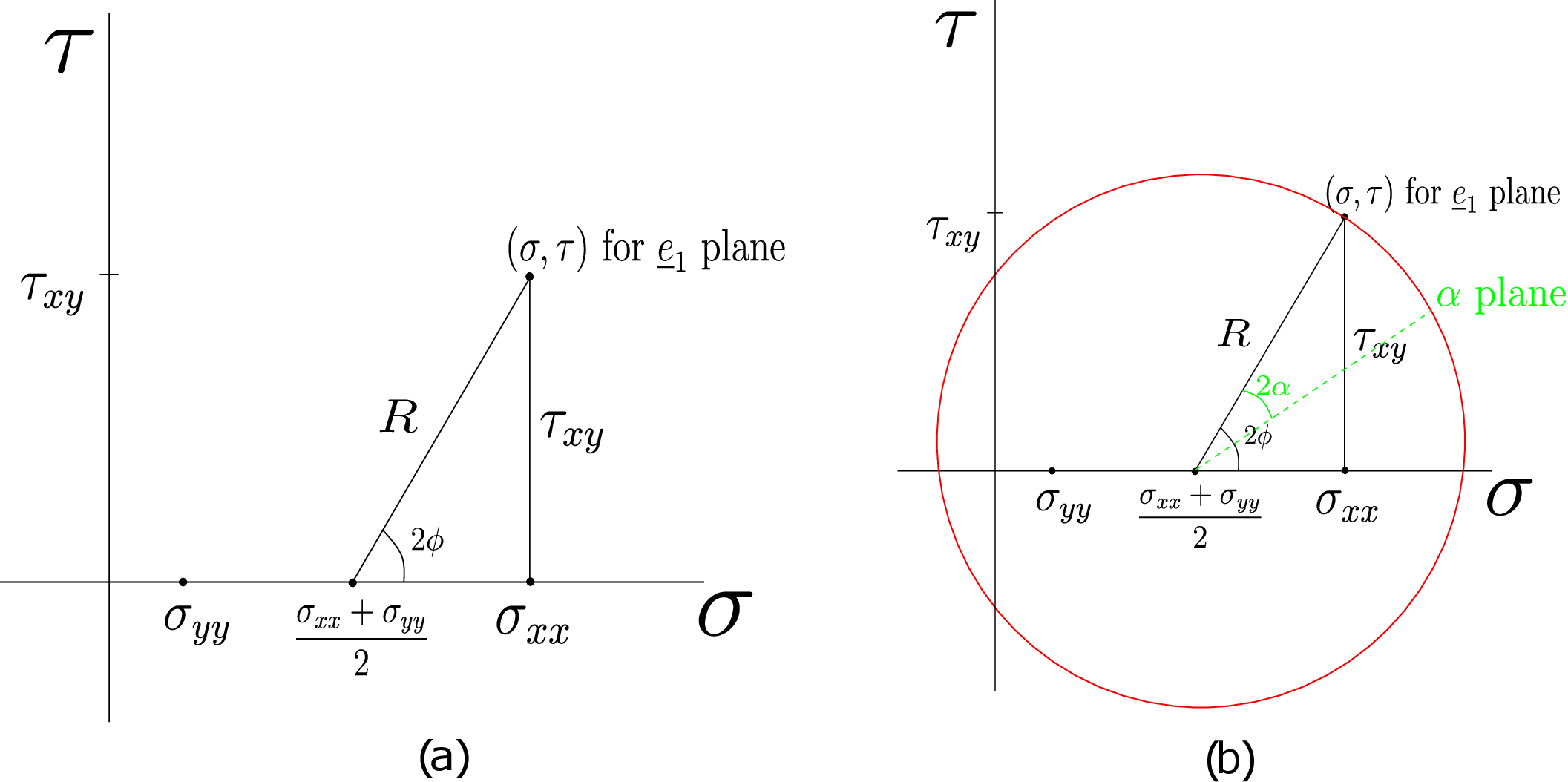
From equation \eqref{4_final_components}, one can make out that by plotting all such points, we will get a circle centered on \(\sigma \) axis at \(\bigg (\dfrac {\sigma _{xx}+\sigma _{yy}}{2},0\bigg )\). Let us start by placing \(\sigma _{xx}\) and \(\sigma _{yy}\) on \(\sigma \) axis. The center of the circle is thus at the mid-point of the two points. We then place \(\tau _{xy}\) on \(\tau \) axis. Now, we can plot the point (\(\sigma _{xx},\tau _{xy}\)) which corresponds to \(\underline {e}_1\) plane. If we join this point with the center, the line obtained will give us the radius of the circle. This is because the circle has to pass through the point corresponding to \(\underline {e}_1\) plane: the circle is the locus of all \((\sigma ,\tau )\) when \(\alpha \) is varied and the point corresponding to \(\underline {e}_1\) plane is obtained for \(\alpha =0\). We can also verify that the radius \(R\) that we obtained graphically also matches with the formula for \(R\) in equation \eqref{4_R}.§ Once we have obtained the radius and center of the circle, we can draw the complete circle as shown in Figure 4.6b. This circle is called the Mohr’s circle. To find \(\sigma \) and \(\tau \) on an arbitrary plane (for general \(\alpha \)), let us look at equation \eqref{4_final_components}: the angle in the cosine and sine terms there is (\(2\phi -2\alpha \)). So, the radial line from the center to the point corresponding to the \(\alpha \)-plane on Mohr’s circle should be at an angle of \((2\phi - 2\alpha )\) from the x-axis. In other words, we can obtain the point corresponding to \(\alpha \)-plane on Mohr’s circle by going in the clockwise direction by angle \(2\alpha \) from the \(\underline {e}_1\)-plane point as shown in green in Figure 4.6b. Let us summarize below the steps involved in drawing the Mohr’s circle and finding the point corresponding to \(\alpha \)-plane:
Notice that the normal to \(\alpha \)-plane is at an angle \(\alpha \) from \(\underline {e}_1\) in counter-clockwise direction (also see Figure 4.4b). But on the Mohr’s circle, we draw that point by rotating by \(2\alpha \) in clockwise direction from the point corresponding to \(\underline {e}_1\)-plane. This is so because in equation \eqref{4_final_components}, we have \(2\alpha \) with a minus sign in the argument of trigonometric functions.
Let us draw the Mohr’s circle again as shown in Figure 4.7.
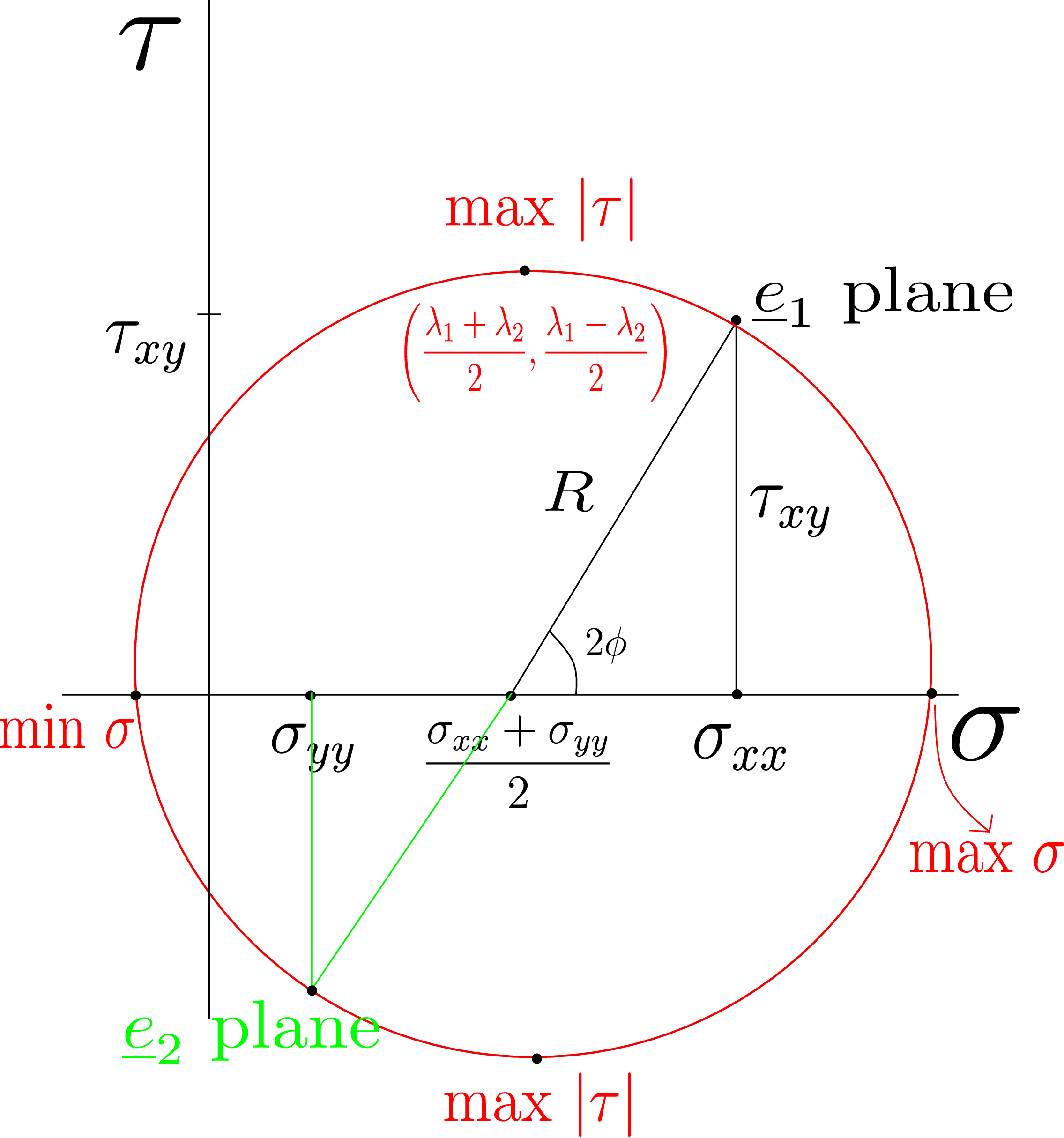
We know the point corresponding to \(\underline {e}_1\) plane. To get to \(\underline {e}_2\) plane, \(\alpha \) should be \(90^{\circ }\) in the counter-clockwise direction. So, in the Mohr’s circle, we need to go \(180^{\circ }\) in the clockwise direction from \(\underline {e}_1\) plane. Thus, we get \(\underline {e}_2\) plane at the diametrically opposite point with respect to \(\underline {e}_1\)-plane point. The two right angled triangles in Figure 4.7 are similar and thus, we get \(\sigma \) at this point as \(\sigma _{yy}\) as required but \(\tau \) as \(-\tau _{xy}\). However, in Figure 4.4b, we see that on \(\underline {e}_2\) plane, shear component is \(\tau _{xy}\). So, why are we getting \(-\tau _{xy}\) from the Mohr’s circle? This is because of our convention for the sign of \(\tau \) as shown on \(\alpha \)-plane in Figure 4.4b - we have defined positive \(\tau \) when we go \(90^{\circ }\) in the counter clockwise direction from the plane normal \(\underline {n}\). For \(\underline {e}_2\) plane, if we go \(90^{\circ }\) in anti-clockwise direction from its plane normal, i.e., \(\underline {e}_2\) direction, we would be pointing along \(-\underline {e}_1\). So, Mohr’s circle is giving us \(\tau \) on \(\underline {e}_2\) plane along \(-\underline {e}_1\) direction whereas \(\tau _{xy}\), by definition, is the shear component along \(+\underline {e}_1\) direction. Therefore, Mohr’s circle gives us \(-\tau _{xy}\) for shear traction on \(\underline {e}_2\) plane. Essentially, we get the negative sign because \(\underline {n}^\perp \) for \(\underline {e}_2\) plane is along \(-\underline {e}_1\) direction.
We can also get the maximum and minimum values of \(\sigma \) and \(\tau \) using Mohr’s circle. The maximum and minimum values of \(\sigma \) are attained on \(\sigma \)-axis itself. These are also shown in Figure 4.7. The maximum and minimum values of \(\tau \) are at the top and bottom of the circle respectively as highlighted in Figure 4.7. We can verify that these values match with the ones derived earlier. Suppose that the principal stress components \(\lambda _1,\lambda _2\) and \(\lambda _3\) are such that \(\lambda _1 > \lambda _2 > \lambda _3\). Thus, \(\lambda _1\) and \(\lambda _2\) correspond to the points of maximum and minimum \(\sigma \), respectively. From the Mohr’s circle, \(\lambda _1\) and \(\lambda _2\) can be obtained by adding and subtracting \(R\) to the \(\sigma \)-value of the circle’s center, respectively, i.e.,
This allows us to get the values of principal stress components directly from the Mohr’s circle: otherwise one has to solve an eigenvalue problem. Writing the center of the circle in terms of principal stress components, we obtain \begin {equation} \text {Center=}\bigg (\frac {\lambda _1+\lambda _2}{2},0\bigg ). \end {equation} We can also get the radius of the circle in terms of principal stress components by subtracting the two principal stress components in equation \eqref{4_principal2}, i.e., \begin {equation} R=\frac {\lambda _{1}-\lambda _{2}}{2}. \end {equation} Remember that in the previous lecture, we had derived the maximum value of shear component of traction to be \(\dfrac {\lambda _{1}-\lambda _{2}}{2}\). And from Mohr’s circle too, we get \(\tau _{\text {max}}=R=\dfrac {\lambda _{1}-\lambda _{2}}{2}\). From the Mohr’s cicrle, we can also see that \(\sigma \) corresponding to the point where we have maximum shear equals the \(\sigma \)-value for the center of the circle, i.e., \(\dfrac {\lambda _{1}+\lambda _{2}}{2}\). This is again the same result that we had derived earlier.
We now want to find the angle of the principal planes from \(x\) plane. We can see in Figure 4.7 that we need to go by an angle of \(2 \phi \) clockwise from \(x\)-plane in the Mohr’s circle to reach the first principal plane, i.e., where \(\lambda _1\) is acting. That means that in the original coordinate system (Figure 4.4b), we need to go by an angle of \(\phi \) in anticlockwise direction from \(x\)-plane to get to the first principal plane. Similarly, for the second principal plane, we have to go \((2 \phi + 180 ^ \circ )\) clockwise in the Mohr’s circle from \(x\)-plane. Thus, in the actual coordinate system we need to go by an angle of \((\phi + 90 ^ \circ )\) in anticlockwise direction from \(\underline {e}_1\) (or \(x\)) plane. Earlier, when we were finding principal planes and principal stress components, we had to solve for the eigenvalues and eigenvectors of the stress matrix. The stress matrix being a \(3\times 3\) matrix, to obtain its eigenvalues, we have to find the roots of its cubic characteristic equation as in equation \eqref{charecteristic_eq_expanded} - this would be mathematically complex and also time consuming when compared to the Mohr’s circle approach. However, the Mohr’s circle procedure has a limitation in that the coordinate system should be chosen in such a way that at least one of the coordinate axes is a principal stress direction.
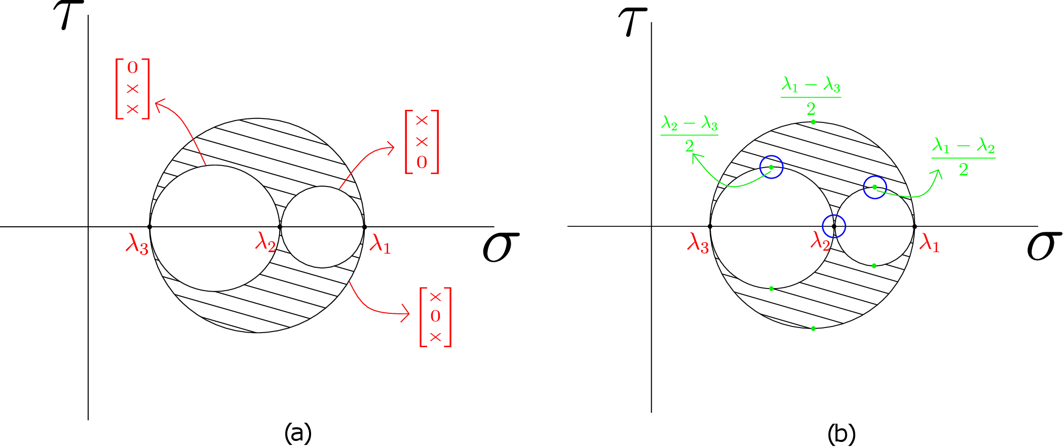
We now move to the next topic: Mohr’s stress plane. Suppose that the stress tensor at a point is such that the three principal stress components are \(\lambda _1\), \(\lambda _2\), \(\lambda _3\) in decreasing order. The stress matrix corresponding to the coordinate system formed by principal directions will be diagonal and given by \begin {equation} \begin {bmatrix} \underline {\underline {\sigma }} \end {bmatrix}= \begin {bmatrix} \lambda _1 & 0 & 0\\ 0 & \lambda _2 & 0\\ 0 & 0 & \lambda _3 \end {bmatrix}. \end {equation} With this stress matrix, suppose we think of arbitrary planes and plot the values of \((\sigma ,\tau )\) on those planes: we are not confining to planes whose normal is perpendicular to one of the principal axes. However, first consider the planes whose normal is perpendicular to \(\underline {e}_3\) axis. If we start plotting \((\sigma ,\tau )\) on such planes, we will get the Mohr’s circle passing through \(\lambda _1\) and \(\lambda _2\) as shown in Figure 4.8.
Similarly, we can draw the Mohr’s circle corresponding to planes whose normals are perpendicular to first principal
axis: this circle passes through \(\lambda _2\) and \(\lambda _3\). Then we take the planes whose normals are perpendicular to second
principal axis: the Mohr’s circle corresponding to such planes passes through \(\lambda _1\) and \(\lambda _3\). This will be the
biggest of the three circles. These three circles correspond to very specific normal directions, i.e., they
have one of their components as zero. These directions are also shown in Figure 4.8a, e.g., the circle
passing through \(\lambda _1\) and \(\lambda _3\) has second component of normal vector as zero. If we now plot \((\sigma ,\tau )\) for all planes
with arbitrary normal directions, we will get the shaded region as shown in Figure 4.8a. The region
within the two inner circles is not realized by any plane. This \(\sigma -\tau \) plot is called the Mohr’s stress plane.
Recall that we had obtained the principal planes by maximizing the normal component of traction. In the process,
we had just set the first derivative of objective function to zero and had not checked the second derivative to identify
whether it’s a minima or maxima or a saddle point. We have in Figure 4.8a a graph where (\(\sigma ,\tau \)) is plotted for all the
planes. With this graph in hand, we can now comment on which of the principal stress components are maxima or
minima: \(\lambda _1\) is the global maxima because the normal component of traction (\(\sigma \)) on this plane is the highest
among all the planes. Likewise \(\lambda _3\) is the global minima. But, \(\lambda _2\) is neither a global maxima nor a global
minima. To see if it is a local maxima or minima, we make a small circle around \(\lambda _2\) as shown in blue in
Figure 4.8b. However small the size of this circle be, it contains points both with higher and lower \(\sigma \)
compared to \(\lambda _2\). Thus, \(\lambda _2\) is neither a local maxima nor a local minima: it is a saddle point. Similarly, we can
comment on the nature of \(\tau _{max}\). We have three \(\tau _{max}\) one for each Mohr’s circle with their magnitudes as \(\dfrac {\lambda _1-\lambda _2}{2}\), \(\dfrac {\lambda _2-\lambda _3}{2}\) and \(\dfrac {\lambda _1-\lambda _3}{2}\)
(shown by green dots in Figure 4.8b). We can immediately see that \(\dfrac {\lambda _1-\lambda _3}{2}\) is the global maxima as no other
plane has \(\tau \) greater than this. The global minimum value of \(\vert \tau \vert \) is zero, so the other two points cannot be
global minima. If we view a small neighbourhood around the other two points shown by blue circles in
Figure 4.8b, we can again conclude that they are neither local maxima or minima. They are also saddle
points.
Consider the special case when two eigenvalues of the stress matrix become same. Let’s say \(\lambda _2=\lambda _3\). So, we have \(\lambda _1 > \lambda _2=\lambda _3\). In the Mohr’s stress plane, the circle corresponding to \((\lambda _2,\lambda _3)\) shrinks to a point while the other inner circle becomes equal to the outer circle (see Figure 4.9a).
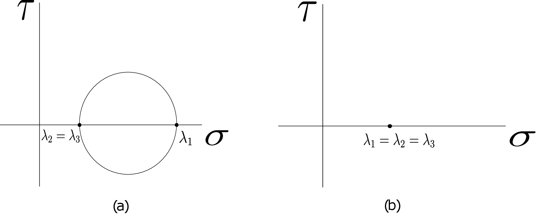
We can visualize this by thinking of \(\lambda _2\) going towards \(\lambda _3\). So, we have just one circle corresponding to \(\lambda _1\) and \(\lambda _2\) and the whole stress plane reduces to a circle.
We can even have a situation where \(\lambda _1 = \lambda _2=\lambda _3\), i.e., all the principal stress components are equal. In this case, the whole region shrinks to a point as shown in Figure 4.9b. So, for any arbitrary plane, we can only have \(\sigma = \lambda _1\) and \(\tau =0\). This situation practically arises in static fluids. Think of a static fluid, say a bucket filled with water as shown in Figure 4.10.
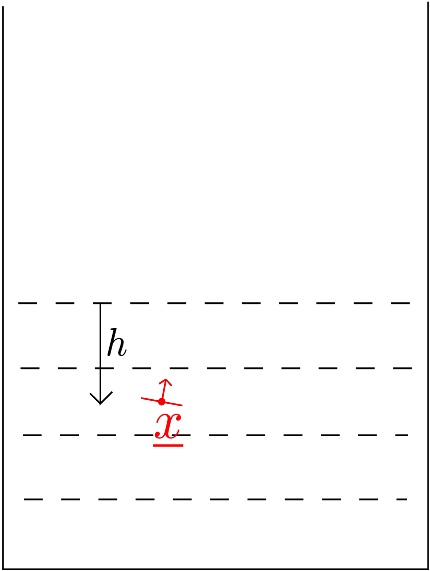
We know that the pressure \(p\) inside water is given by \(\rho g h\) where \(h\) is the depth from the top surface, \(g\) is the acceleration due to gravity and \(\rho \) is the density of water. However, what is the state of stress at any point in the water body? Let us think of an infinitesimal plane at an arbitrary point \(\underline {x}\) in the fluid (see Figure 4.10). As fluids cannot sustain shear when they are in static equilibrium, there will be no shear component of traction on this plane. In fact, the traction would be the same as the pressure \(p\) and acting along the plane normal but pointing into the plane due to compressive nature of pressure. Thus, at an arbitrary point \(\underline {x}\) in the fluid and on an arbitrary plane (say having plane normal \(\underline {n}\)), traction \(\underline {t}\) will be given by \begin {equation} \label {traction_fluid} \underline {t}(\underline {x};\underline {n})=-p(\underline {x})~\underline {n}. \end {equation} To obtain stress tensor, we can rewrite the above equation as follows: \begin {equation} \underline {t}=-p~ \underline {n}=-p\underline {\underline {I}}\,\underline {n}\Rightarrow \underline {\underline {\sigma }}=-p\underline {\underline {I}}. \end {equation} Thus, the stress tensor for a fluid body in statics is \(-p\underline {\underline {I}}\). The corresponding stress matrix say in (\(\underline {e}_1\), \(\underline {e}_2\), \(\underline {e}_3\)) coordinate system can be found easily. The traction on \(\underline {e}_{i}\) plane will be \(-p\underline {e}_i\). So \begin {equation} [\underline {\underline {\sigma }}]_{(\underline {e}_1, \underline {e}_2, \underline {e}_3)}= \begin {bmatrix} -p & 0 & 0\\ 0 & -p & 0\\ 0 & 0 & -p \end {bmatrix}=-p \begin {bmatrix} \underline {\underline {I}} \end {bmatrix}. \end {equation} This state of stress is also called the hydrostatic state of stress (‘static’ because the fluid is in statics). We also have \(\lambda _1 = \lambda _2=\lambda _3 = -p\).
As the body deforms, stress develops at every point in the body. The corresponding stress matrix at a point depends on the choice of the coordinate system. We had also derived the following transformation law that transforms the stress matrix from one coordinate system into another: \begin {equation} \label {sigma_transformation} \begin {bmatrix} \underline {\underline {\hat \sigma }} \end {bmatrix}= \begin {bmatrix} \underline {\underline {R}} \end {bmatrix}^T \begin {bmatrix} \underline {\underline {\sigma }} \end {bmatrix} \begin {bmatrix} \underline {\underline {R}} \end {bmatrix}. \end {equation} Here \(\begin {bmatrix}\underline {\underline {R}}\end {bmatrix}\) represents the matrix form of rotation tensor that transforms the initial coordinate axes to the new ones while \(\begin {bmatrix}\underline {\underline {\hat \sigma }}\end {bmatrix}\) and \(\begin {bmatrix}\underline {\underline {\sigma }}\end {bmatrix}\) denote stress matrices in new and old coordinate systems respectively. The above relation implies that individual components of stress matrix change with coordinate system but there are some quantities that do not change. For example, we have learnt about principal stress components. They are obtained as the eigenvalues of the stress matrix. We will show now that principal planes and principal stress components are independent of the coordinate system. We have the following eigenvalue-eigenvector equation for the stress matrix:
The determinant of the matrix in parentheses is then equated to zero to get eigenvalues, i.e., \begin {equation} \label {4_characteristic_equation} det\Big [\underline {\underline {\sigma }}-\lambda \, \underline {\underline {I}}\Big ]=0. \end {equation} This yields a cubic equation in \(\lambda \) (also called the characteristic equation) solving which we obtain all the eigenvalues. Let us obtain this equation for the transformed matrix. We thus have
We know that the determinant of product of matrices is the same as the product of determinant of matrices. Also, rotation matrix being orthonormal, its determinant equals 1. Thus, the above equation further becomes
Thus, we get the same characteristic equation as in \eqref{4_characteristic_equation}. This proves that the eigenvalues and hence principal stress components are invariant. Indeed, that is also expected since principal stress components are also the properties of the stress tensor. Let us now write equation \eqref{4_characteristic_equation} in component form, we get \begin {equation} det\begin {bmatrix} \sigma _{11}-\lambda & \sigma _{12} &\sigma _{13}\\ \sigma _{12} & \sigma _{22}-\lambda &\sigma _{23}\\ \sigma _{13} & \sigma _{23} &\sigma _{33}-\lambda \end {bmatrix}=0. \end {equation} Upon further expanding the determinant, we get \begin {equation} \label {charecteristic_eq_expanded} -\lambda ^3 +\lambda ^2(\sigma _{11}+\sigma _{22}+\sigma _{33})-\lambda ( \sigma _{22}\sigma _{33}+\sigma _{11}\sigma _{33}+\sigma _{11}\sigma _{22}-\sigma _{12}^2-\sigma _{13}^2-\sigma _{23}^2)+det\big (\underline {\underline {\sigma }}\big )=0. \end {equation} This is the characteristic equation (cubic in eigenvalue) in terms of matrix components. A cubic equation, in general, can also have imaginary roots. But here, we know that this equation corresponds to the symmetric stress matrix which always has 3 principal stress components. The characteristic equation in the hat coordinate system will be the following: \begin {equation} -\lambda ^3 +\lambda ^2(\hat \sigma _{11}+\hat \sigma _{22}+\hat \sigma _{33})-\lambda ( \hat \sigma _{22}\hat \sigma _{33}+\hat \sigma _{11}\hat \sigma _{33}+\hat \sigma _{11}\hat \sigma _{22}-\hat \sigma _{12}^2-\hat \sigma _{13}^2-\hat \sigma _{23}^2)+det\big (\underline {\underline {\hat \sigma }}\big )=0. \end {equation} However, as the three roots have to be the same, the coefficients of this equation must be the same in any coordinate system. Thus, the coefficients of the characteristic equation are also the invariants and are called \(I_1,I_2\) and \(I_3\) as shown below: \begin {equation} -\lambda ^3 +\lambda ^2\underbrace {(\sigma _{11}+\sigma _{22}+\sigma _{33})}_{I_1}-\lambda \underbrace {( \sigma _{22}\sigma _{33}+\sigma _{11}\sigma _{33}+\sigma _{11}\sigma _{22}-\sigma _{12}^2-\sigma _{13}^2-\sigma _{23}^2)}_{I_2}+\underbrace {det\big (\underline {\underline {\sigma }}\big )}_{I_3}=0. \end {equation} The expression of these three coefficients become simple if they are obtained from the stress matrix in the coordinate system of principal directions, i.e.,
The simplification happened because the matrix has no shear component in the coordinate system of principal directions. We can also notice that \(I_1\) is the sum of the roots, \(I_2\) is the sum of the three combinations of pair products of roots and \(I_3\) is the product of the three roots.
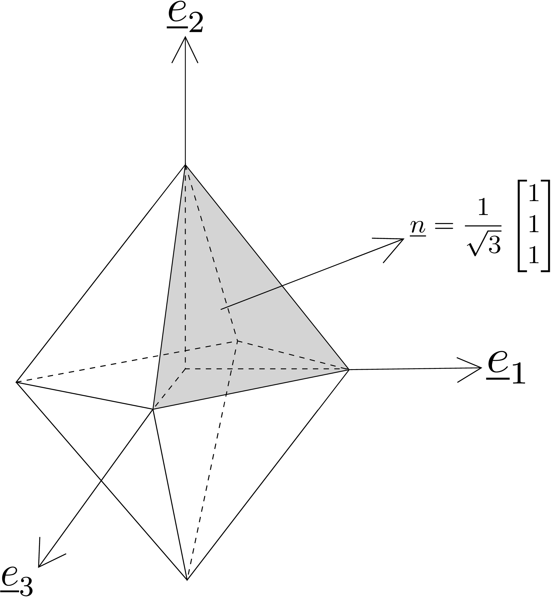
To define octahedral stress components, we need to know what an octahedral plane is: they are the faces of an octahedron having 8 faces whose normals have the following form \begin {equation} \label {4_normal_octahedral} \begin {bmatrix} \underline {n} \end {bmatrix}= \begin {bmatrix} \frac {\pm 1}{\sqrt {3}}\\ \frac {\pm 1}{\sqrt {3}}\\ \frac {\pm 1}{\sqrt {3}} \end {bmatrix} \end {equation} in the coordinate system of principal directions, i.e., they are equally inclined from all principal directions. Let us consider the octahedron shown in Figure 4.11. The normal and shear components of traction on its octahedral faces are called octahedral stress components. The normal component of traction on octahedral planes (denoted by \(\sigma _{oct}\)) will be
which turns out to be an invariant. Its expression in terms of components of a general stress matrix becomes \begin {equation} \sigma _{oct}=\frac {\sigma _{11}+\sigma _{22}+\sigma _{33}}{3}. \end {equation} Similarly, we can find \(\tau _{oct}\) as follows:
which again turns out to be an invariant. Also, note that irrespective of what face out of the 8 octahedral planes we take, we have the same \(\sigma _{oct}\) and \(\tau _{oct}\). We will see their significance later on when we discuss various failure theories.
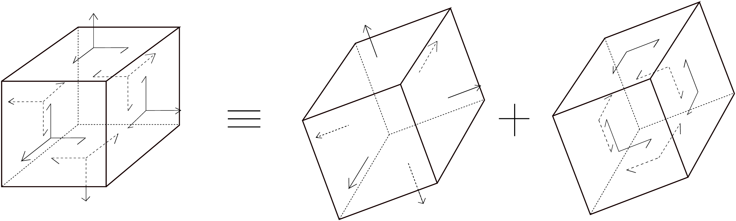
We can additively decompose an arbitrary stress tensor into hydrostatic and deviatoric parts. Consider adding and subtracting \(\dfrac {1}{3}I_1(\underline {\underline {\sigma }})~\underline {\underline {I}}\) to a general stress tensor \(\underline {\underline {\sigma }}\) as shown below: \begin {equation} \label {stress_breakdown} \underline {\underline {\sigma }}=\frac {1}{3}I_1(\underline {\underline {\sigma }}) ~\underline {\underline {I}}+\Big (\underline {\underline {\sigma }}-\frac {1}{3}I_1(\underline {\underline {\sigma }}) ~\underline {\underline {I}}\Big ). \end {equation} Let us denote the part within the parantheses as \(\underline {\underline {\hat \sigma }}\). This is a special kind of decomposition because the first term is proportional to the identity tensor whereas the second term is such that its first invariant is 0 which can be proved as follows: \begin {equation} I_1\Big (\underline {\underline {\hat \sigma }}\Big )=I_1\Big (\underline {\underline {\sigma }}\Big )-I_1\Big (\frac {1}{3}I_1(\underline {\underline {\sigma }})~ \underline {\underline {I}}\Big )=I_1\Big (\underline {\underline {\sigma }}\Big )-\frac {1}{3}I_1(\underline {\underline {\sigma }})~I_1(\underline {\underline {I}})=0. \end {equation} Due to this property, \(\underline {\underline {\hat \sigma }}\) is also called the deviatoric part of stress tensor whereas the first term that is proportional to identity is called the hydrostatic part of stress tensor. There is a physical reason for calling the second term the deviatoric part. There always exists a special coordinate system such that the matrix form of the deviatoric part has all its diagonal entries zero, i.e., \(\underline {\underline {\hat \sigma }}\) has the following matrix form: \begin {equation} \label {4_diagonal_zero} \begin {bmatrix} \underline {\underline {\hat \sigma }} \end {bmatrix}= \begin {bmatrix} 0 & \times & \times \\ \times & 0 & \times \\ \times & \times & 0 \end {bmatrix} \end {equation} As diagonal elements of the stress matrix are zero, there will be no normal traction on the three planes whose normals are aligned with the coordinate axes of this special coordinate system. These planes only have shear traction. If we visualize the cuboid corresponding to this coordinate system, the faces of the cuboid will be under pure shear which will just try to change/distort the shape of the cuboid keeping its volume fixed (see Figure 4.12). This is why we call it the deviatoric part of stress tensor. A stress matrix of such a kind as in equation \eqref{4_diagonal_zero} is also said to correspond to the state of pure shear. On the other hand, the hydrostatic part leads to only normal traction acting on the faces of the cuboid. This normal traction will be the same on all the faces and so, it just tries to change the size of the cuboid without distorting its shape.
Q1. A cylindrical rod is subjected to a torque T at both its ends. Its lateral surface is assumed to be traction free. We will learn later that at any point in its cross-section, the following stress components exist: \[\sigma _{xx}=\sigma _{yy}=\sigma _{zz}=\tau _{xy}=\tau _{yx}=0, \; \tau _{xz}=\tau _{zx}=-G\kappa {y},\; \tau _{yz}=\tau _{zy}=G\kappa {x}.\]
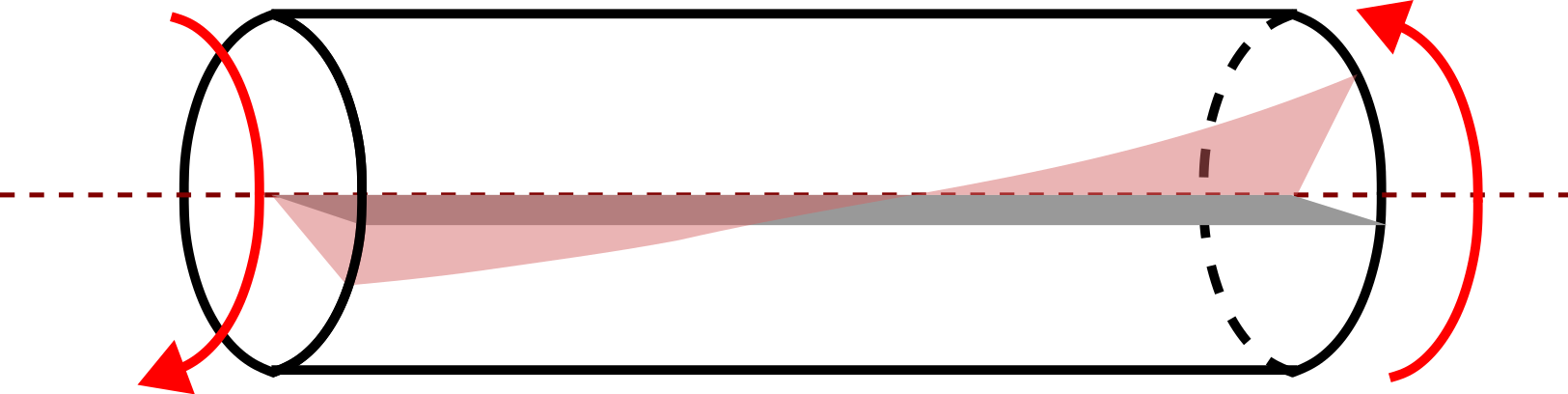
Here \(G\) is a material parameter and \(\kappa \) is the twist induced in the rod due to torque. Also, z-axis lies along the length of the beam. Determine the principal stress components, maximum shear stress values and the associated plane normals on which they are realized.
Solution: We cannot apply Mohr’s circle concept here since none of the coordinate axis is a principal axis. Accordingly, we will have to solve the eigenvalue-eigenvector problem. To obtain the principal stress components, we first set \(\det \brc {\sbk {\matr {\sigma }} - \lambda \sbk {\matr {\text {I}}}} = 0\) and obtain the characteristic equation: \begin {align*} \det \brc {\begin {bmatrix} -\lambda & 0 & -G \theta y \\ 0 & -\lambda & G \theta x \\ -G \theta y & G \theta x & -\lambda \end {bmatrix}} &= 0 \Rightarrow -\lambda ^3 + \lambda G^2 \theta ^2 \brc {x^2 + y^2} &= 0~ \text {or}~ \lambda \brc {\lambda ^2 - G^2 \theta ^2 \brc {x^2 + y^2}} = 0. \end {align*}
Therefore, we get the principal stress components to be (in decreasing order): \[\lambda _1 = G\theta \sqrt {x^2 + y^2}, \quad \lambda _2 = 0, \quad \lambda _3 = - G\theta \sqrt {x^2 + y^2}.\] The first principal stress plane can be found as follows: \begin {align*} \begin {bmatrix} -\lambda _1 & 0 & -G \theta y \\ 0 & -\lambda _1 & G \theta x \\ -G \theta y & G \theta x & -\lambda _1 \end {bmatrix} \begin {bmatrix} n^1_{1} \\ n^1_{2} \\ n^1_3 \end {bmatrix} &= \begin {bmatrix} 0 \\ 0 \\ 0 \end {bmatrix}. \end {align*}
Below we write the three equations (of which only two are independent) plus one equation for the normalization of the normal vector: \begin {align*} -\lambda _1 n^1_{1} - G \theta y \; n^1_{3} &= 0, \\ -\lambda _1 n^1_{2} - G \theta x \; n^1_{3} &= 0, \\ -G \theta y \; n^1_{1} - G \theta x \; n^1_{2} - \lambda _1 n^1_3 &= 0, \\ \brc {n^1_1}^2 + \brc {n^1_2}^2 + \brc {n^1_3}^2 &= 1. \end {align*}
Solving the above set of equations, we get \begin {align*} n^1_3 = \pm \frac {1}{\sqrt {2}}, ~ n^1_1 = \mp \frac {y}{\sqrt {2(x^2+y^2)}}, n^1_2 = \mp \frac {x}{\sqrt {2(x^2+y^2)}}. \end {align*}
Similarly, one can also solve for the normals corresponding to other two principal stress components (not worked out here). One of them will be the radial direction corresponding to zero principal stress component. The third one will be perpendicular to other two. For the maximum shear stresses, we get \[\tau _1 = \abs {\frac {\sigma _{11} - \sigma _{33}}{2}} = G\theta \sqrt {x^2+y^2},\] \[\tau _2 = \abs {\frac {\sigma _{11} - \sigma _{22}}{2}} = \frac {1}{2}G\theta \sqrt {x^2+y^2}, ~ \tau _3 = \abs {\frac {\sigma _{22} - \sigma _{33}}{2}} = \frac {1}{2}G\theta \sqrt {x^2+y^2}. \]
Q2. Suppose the stress matrix in a given coordinate system is given by \begin {equation} \label {4_stress_matrix} \begin {bmatrix} \underline {\underline {\sigma }} \end {bmatrix}= \begin {bmatrix} 4 \sqrt {2}& 2 \sqrt {2} &0\\ 2 \sqrt {2} & 8 \sqrt {2} &0\\ 0 & 0 &10 \end {bmatrix}.\nonumber \end {equation} Illustrate the application of Mohr’s circle for this stress matrix.
Let us find the principal planes, the plane corresponding to maximum shear stress, values of principal stress components and the maximum shear stress. We can immediately see from the stress matrix that \(\underline {e}_3\) axis is aligned with the principal axis and hence we can use Mohr’s circle analysis here. On \(\sigma -\tau \) plane, we first plot \(\sigma _{xx}\) and \(\sigma _{yy}\). The center of the circle will be at the mid point of these two, i.e., at \(6 \sqrt {2}\) on the \(\sigma \) axis. Then we plot the point corresponding to \(\underline {e}_1\) plane which is (\(4 \sqrt {2},2 \sqrt {2}\)). Now we can join the center and the point corresponding to \(\underline {e}_1\) plane to get radius. Using Pythagoras theorem: \begin {equation} R=\sqrt {(2 \sqrt {2})^2+(2 \sqrt {2})^2}=4.\nonumber \end {equation} With this radius and the center known, we draw our Mohr’s circle as shown in Figure ??.
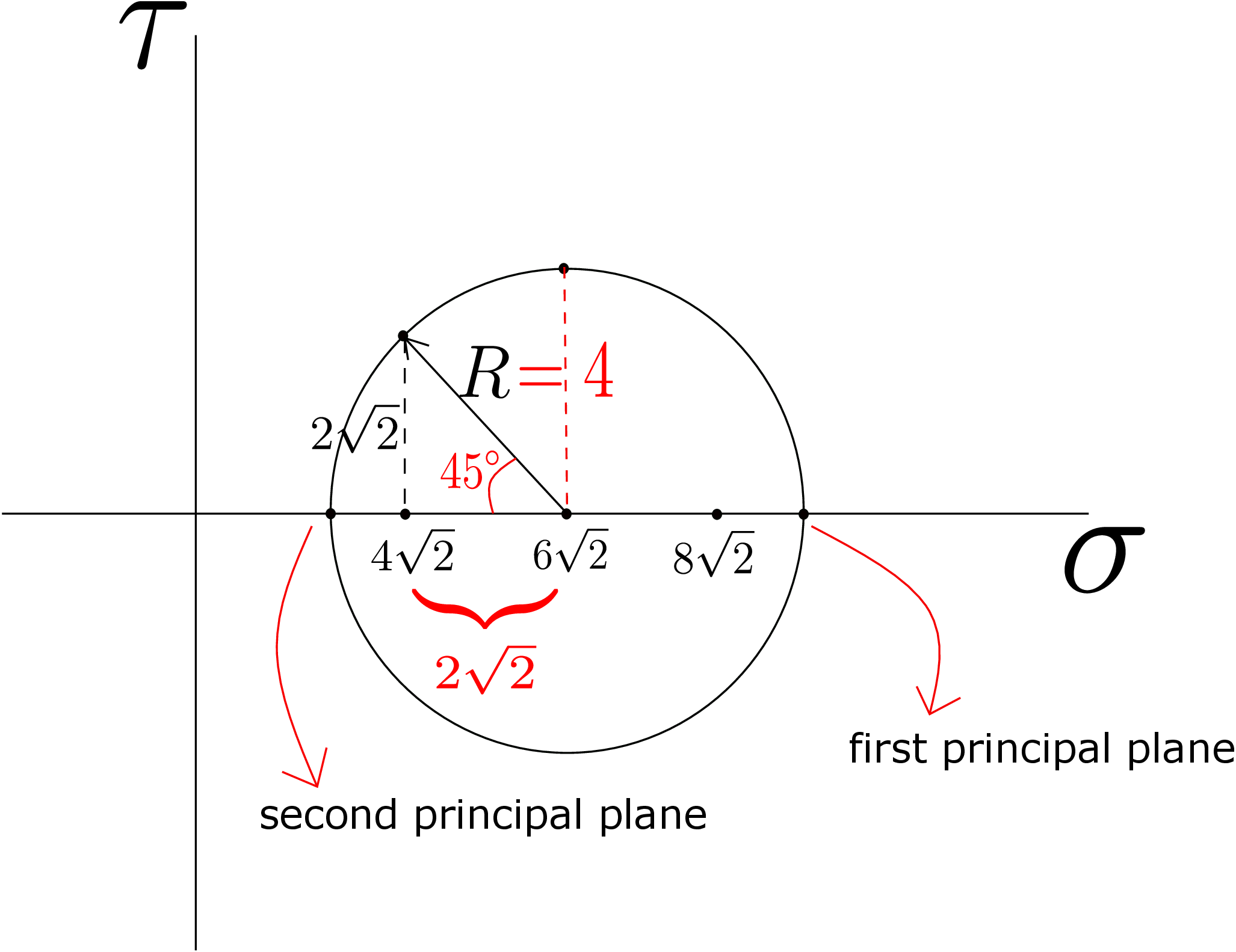
We can see that the principal stress components and \(\tau _{max}\) are:
We now want to find the orientation of principal plane having principal component as \((6 \sqrt {2}+4)\). In the Mohr’s circle, we need to find the angle of the point corresponding to this plane with the point representing \(\underline {e}_1\) plane. Both the sides of the right angled triangle shown are \(2 \sqrt {2}\), thus making it an isosceles triangle. Thus, we have to go \(135 ^ \circ \) clockwise on the Mohr’s circle to get to the first principal plane. So, in the actual coordinate system, we have to go \(\bigg (\dfrac {135}{2}\bigg ) ^ \circ \) counterclockwise. Similarly, we can find the angle for the second principal plane. For the plane having maximum shear, we need to rotate by \(45 ^ \circ \) clockwise on the Mohr’s circle. So in the actual coordinate system, we need to go \(\bigg (\dfrac {45}{2}\bigg ) ^ \circ \) counterclockwise.
For an exhaustive set of solved examples and unsolved objective and subjective type questions, please refer to the printed book.
∗In this formulation, the three components of the normal direction are assumed to be independent of each other and the constraint equation automatically takes care of the relevant relation between them.
†Note that two vertical bars on each side are used to denote magnitude of a vector whereas single vertical bar on each side is used to denote magnitude of a scalar.
‡Notice that we have taken only one out of \(n_1\), \(n_2\) and \(n_3\) to be zero. If we take two of them to be zero, the magnitude condition binds the third to be 1. This will give us the direction corresponding to principal plane where shear component is zero. In other words, this direction yields minima of \(\tau ^2\) which is not of interest.
§The right angled triangles in Figures 4.5 and 4.6a turn out to be the same!