3 Stress Equilibrium Equations

Chapter 3
Stress Equilibrium Equations

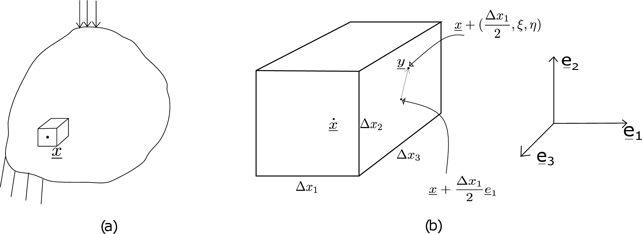
Suppose we have a body which is clamped at some part of its boundary and further subjected to external load at other part of its boundary (see Figure 3.1a).

Figure 3.1: (a) A body under the action of some applied load: a cuboidal region is considered in the body with its center at \(\underline {x}\) (b) zoomed view of the cuboid: the coordinates of an arbitrary point \(\underline {y}\) on the cuboid’s +ve \(\underline {e}_1\) face is shown

We have talked about traction vector and stress tensor at a point in the body but not how they vary in the body. Due to externally applied load, stress is induced in the body which, in general, varies in the body from point to point. To know where the body would fail, we would need to know the value of stress components at every point in the body. The stress equilibrium equations allow us to obtain this distribution of stress and ultimately helps in designing against failure. Let us know derive these equations.

3.1 Linear momentum balance: NPTEL link

We begin with applying balance of linear momentum to an arbitrary part of the body. Think of a small cuboidal region in the body with its centroid at \(\underline {x}\) (see Figure 3.1a). Further, suppose the edges of this cuboid are aligned along \(\underline {e}_1, \underline {e}_2\) and \(\underline {e}_3\) directions with their lengths being \(\Delta x_1\), \(\Delta x_2\) and \(\Delta x_3\) respectively (see Figure 3.1b). Let us apply Newton’s second law to the mass contained in this cuboid, i.e., \begin {equation} \label {3_newton_law} \sum \underline {F}^{ext}=\frac {d}{dt}\underline {P} \end {equation} where \(\underline {P}\) denotes the total linear momentum of the mass within the cuboid. To find net external force on this cuboid, we need to sum all the forces acting on it due to tractions and body force. Let us obtain the traction contribution first.

Starting with \(\underline {e}_1\)-plane, an arbitrary point on this face will have its position at \(\underline {x}+\)\(\left ( \dfrac {\Delta x_1}{2},\xi ,\eta \right )\) (see Figure 3.1b). This is because we need to move by \(\dfrac {\Delta x_1}{2} \underline { e}_1\) from the centroid to first reach the center of the \(\underline {e}_1\)-face. Then, any arbitrary point on this face will have some coordinate along \(\underline {e}_2\) and \(\underline {e}_3\) given by \(\xi \) and \(\eta \), respectively. In general, traction will vary from point to point on this face. For the particular point under consideration, traction will be given by \begin {equation} \label {traction_e_1} \underline {t}^1(\underline {x} +\dfrac {\Delta x_1}{2} \underline { e}_1+\xi \underline {e}_2+\eta \underline {e}_3)= \underline {\underline {\sigma }}(\underline {x} +\dfrac {\Delta x_1}{2} \underline { e}_1+\xi \underline {e}_2+\eta \underline {e}_3)~\underline {e}_1. \end {equation} Let us write this in terms of the stress tensor at the centroid of the cuboid. One can use Taylor’s expansion as shown below: \begin {equation} \label {taylor_expansion} \underline {\underline {\sigma }}(\underline {x} +\dfrac {\Delta x_1}{2} \underline { e}_1+\xi \underline {e}_2+\eta \underline {e}_3)~\underline {e}_1= \Bigg [\underline {\underline {\sigma }}+\dfrac {\partial \underline {\underline {\sigma }}}{\partial x_1}\dfrac {\Delta x_1}{2}+\dfrac {\partial \underline {\underline {\sigma }}}{\partial x_2}\xi +\dfrac {\partial \underline {\underline {\sigma }}}{\partial x_3}\eta +.....\Bigg ]\underline {e}_1. \end {equation} Keep in mind that \(\underline {\underline {\sigma }}\) and its derivatives on the right hand side of the above equation are evaluated at the cuboid’s centroid. The total force due to traction on \(\underline {e}_1\) plane will be obtained by integration of traction over the area of this plane. As \(\xi =0\) and \(\eta =0\) corresponds to the center of this surface, we need to integrate from \(\dfrac {-\Delta x_2}{2}\) to \(\dfrac {\Delta x_2}{2}\) for \(\xi \) and from \(\dfrac {-\Delta x_3}{2}\) to \(\dfrac {\Delta x_3}{2}\) for \(\eta \). Thus \begin {equation} \label {force_e_1} \underline {F}^{1}=\int \limits _{\tfrac {-\Delta x_3}{2}}^{\tfrac {\Delta x_3}{2}}\int \limits _{\tfrac {-\Delta x_2}{2}}^{\tfrac {\Delta x_2}{2}}\underline {t}^1 d\xi d\eta =\int \limits _{\tfrac {-\Delta x_3}{2}}^{\tfrac {\Delta x_3}{2}}\int \limits _{\tfrac {-\Delta x_2}{2}}^{\tfrac {\Delta x_2}{2}}\Bigg [\underline {\underline {\sigma }}+\dfrac {\partial \underline {\underline {\sigma }}}{\partial x_1}\dfrac {\Delta x_1}{2}+\dfrac {\partial \underline {\underline {\sigma }}}{\partial x_2}\xi +\dfrac {\partial \underline {\underline {\sigma }}}{\partial x_3}\eta \Bigg ]\underline {e}_1 d\xi d\eta . \end {equation} The first two terms within square brackets in the above equation are independent of \(\xi \) and \(\eta \). So, they can be taken out of the integration and integration of the remaining term simply gives the total area of \(\underline {e}_1\) face. The third term is independent of \(\eta \) and the fourth is independent of \(\xi \). So, we get \begin {equation} \underline {F}^{1}=\Bigg [\underline {\underline {\sigma }}+\dfrac {\partial \underline {\underline {\sigma }}}{\partial x_1}\dfrac {\Delta x_1}{2}\Bigg ]\underline {e}_1\Delta x_2\Delta x_3+ \dfrac {\partial \underline {\underline {\sigma }}}{\partial x_2}\underline {e}_1\Delta x_3\int \limits _{\tfrac {-\Delta x_2}{2}}^{\tfrac {\Delta x_2}{2}}\xi d\xi + \dfrac {\partial \underline {\underline {\sigma }}}{\partial x_3}\underline {e}_1\Delta x_2\int \limits _{\tfrac {-\Delta x_3}{2}}^{\tfrac {\Delta x_3}{2}}\eta d\eta . \end {equation} The two single integrals above can be shown to vanish. On further noting that \(\Delta x_1\Delta x_2\Delta x_3\) is the volume of the cuboid (denoted by \(\Delta V\)), we obtain \begin {equation} \label {force_e_plus1} \underline {F}^1=\underline {\underline {\sigma }}~\underline {e}_1\Delta x_2\Delta x_3 +\dfrac {\partial \underline {\underline {\sigma }}}{\partial x_1}\underline {e}_1\dfrac {\Delta V}{2}. \end {equation} The force on \(-\underline {e}_1\) plane will likewise be

\begin {eqnarray} \underline {F}^{-1}=\int \limits _{\tfrac {-\Delta x_3}{2}}^{\tfrac {\Delta x_3}{2}}\int \limits _{\tfrac {-\Delta x_2}{2}}^{\tfrac {\Delta x_2}{2}} \underline {t}^{-1}d\xi d\eta &=&\int \limits _{\tfrac {-\Delta x_3}{2}}^{\tfrac {\Delta x_3}{2}}\int \limits _{\tfrac {-\Delta x_2}{2}}^{\tfrac {\Delta x_2}{2}}\Bigg [\underline {\underline {\sigma }}(\underline {x}-\dfrac {\Delta x_1}{2} \underline {e}_1+\xi \underline {e}_2+\eta \underline {e}_3)\Bigg ](-\underline {e}_1) d\xi d\eta \nonumber \\ &=&\int \limits _{\tfrac {-\Delta x_3}{2}}^{\tfrac {\Delta x_3}{2}}\int \limits _{\tfrac {-\Delta x_2}{2}}^{\tfrac {\Delta x_2}{2}}\Bigg [\underline {\underline {\sigma }}-\dfrac {\partial \underline {\underline {\sigma }}}{\partial x_1}\dfrac {\Delta x_1}{2}+\dfrac {\partial \underline {\underline {\sigma }}}{\partial x_2}\xi +\dfrac {\partial \underline {\underline {\sigma }}}{\partial x_3}\eta \Bigg ](-\underline {e}_1)d\xi d\eta \nonumber \\ &=&-\underline {\underline {\sigma }}~\underline {e}_1\Delta x_2\Delta x_3 +\dfrac {\partial \underline {\underline {\sigma }}}{\partial x_1}\underline {e}_1\dfrac {\Delta V}{2}.\label {force_e_minus1} \end {eqnarray}

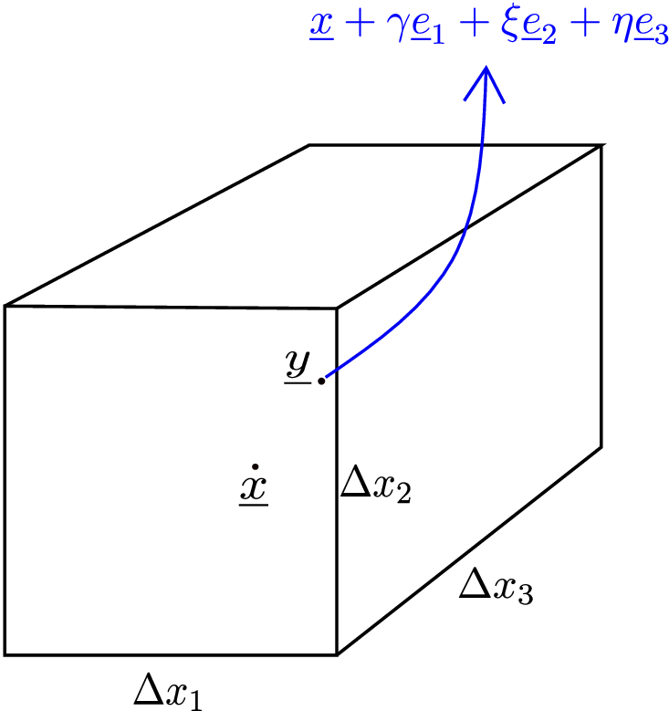
The total force on \(\underline {e}_1\) and -\(\underline {e}_1\) faces is thus \begin {equation} \label {3_total_e_1} \underline {F}^1+\underline {F}^{-1}=\dfrac {\partial \underline {\underline {\sigma }}}{\partial x_1}\underline {e}_1~\Delta V. \end {equation} We can then find out the total force on \(+\underline {e}_2\) and \(-\underline {e}_2\) planes using similar analysis and we will find that only the index ‘1’ changes to ‘2’ in equation \eqref{3_total_e_1}. Similarly, for total force on \(+\underline {e}_3\) and \(-\underline {e}_3\) planes, the index ‘1’ changes to ‘3’. Accordingly, the total traction force (denoted by \(\underline {F}^{tra}\)) on all the six faces will be \begin {equation} \label {3_total_traction_force} \underline {F}^{tra}=\sum _{i=1}^3 \dfrac {\partial \underline {\underline {\sigma }}}{\partial x_i}\underline {e}_i~\Delta V. \end {equation} Let us now obtain the body force contribution. We denote the body force by \(\underline {b}\) which will, in general, be a function of the position vector of the point where it is acting. A general point in the cuboid has its position vector (\(\underline {x}+\gamma \underline {e}_1+\xi \underline {e}_2+\eta \underline {e}_3\)) - see Figure 3.2. Thus, the total body force would be

\begin {eqnarray} \underline {F}^b &=&\int \limits _{\tfrac {-\Delta x_1}{2}}^{\tfrac {\Delta x_1}{2}}\int \limits _{\tfrac {-\Delta x_2}{2}}^{\tfrac {\Delta x_2}{2}}\int \limits _{\tfrac {-\Delta x_3}{2}}^{\tfrac {\Delta x_3}{2}}\underline {b}(\underline {x}+\gamma \underline {e}_1+\xi \underline {e}_2+\eta \underline {e}_3)~d\gamma d\xi d\eta \nonumber \\ &=&\int \limits _{\tfrac {-\Delta x_1}{2}}^{\tfrac {\Delta x_1}{2}}\int \limits _{\tfrac {-\Delta x_2}{2}}^{\tfrac {\Delta x_2}{2}}\int \limits _{\tfrac {-\Delta x_3}{2}}^{\tfrac {\Delta x_3}{2}}\Bigg [\underline {b}+\dfrac {\partial \underline {b}}{\partial x_1}\gamma +\dfrac {\partial \underline {b}}{\partial x_2}\xi +\dfrac {\partial \underline {b}}{\partial x_3}\eta +....\Bigg ]d\gamma d\xi d\eta \nonumber ~(\text {using Taylor's expansion})\\ &=&\underline {b}~\Delta V+\dfrac {\partial \underline {b}}{\partial x_1}\Delta x_2\Delta x_3\int \limits _{\tfrac {-\Delta x_1}{2}}^{\tfrac {\Delta x_1}{2}}\gamma d\gamma + \dfrac {\partial \underline {b}}{\partial x_2}\Delta x_1\Delta x_3\int \limits _{\tfrac {-\Delta x_2}{2}}^{\tfrac {\Delta x_2}{2}}\gamma d\gamma + \dfrac {\partial \underline {b}}{\partial x_3}\Delta x_1\Delta x_2\int \limits _{\tfrac {-\Delta x_3}{2}}^{\tfrac {\Delta x_3}{2}}\gamma d\gamma \nonumber +o(\Delta V)\\ &=&\underline {b}~\Delta V+0+0+0+o(\Delta V)\nonumber \\ &=&\underline {b}~\Delta V+o(\Delta V).\label {3_total_body_force} \end {eqnarray}

Here \(o(\Delta V)\) denotes the integration of higher order terms in the above Taylor’s expansion. It is a formal notation in mathematics and is pronounced as ‘small oh’. It means that if \(\Delta V\) approaches zero then \(o(\Delta V)\) term goes to zero faster than \(\Delta V\), i.e., \begin {equation} \label {3_small_order_terms} \lim _{\Delta V \to 0} \frac {o(\Delta V)}{\Delta V}=0. \end {equation} Let us now obtain the RHS of equation \eqref{3_newton_law}. We first obtain the total linear momentum \(\underline {P}\) by integrating linear momentum of infinitesimal masses in the cuboid, i.e., \begin {equation} \underline {P}=\int \int \int dm\hspace {1mm}\underline {v}=\int \int \int (\rho dV)~\underline {v}=\int \limits _{\tfrac {-\Delta x_3}{2}}^{\tfrac {\Delta x_3}{2}}\int \limits _{\tfrac {-\Delta x_2}{2}}^{\tfrac {\Delta x_2}{2}}\int \limits _{\tfrac {-\Delta x_1}{2}}^{\tfrac {\Delta x_1}{2}}\rho \underline {v}\hspace {1mm}d\gamma d\xi d\eta . \end {equation} As the velocity and density could be varying arbitrarily within the cuboid, we again need to use Taylor’s expansion of \(\rho \underline {v}\) about the centroid. When we use this expansion and evaluate the integration similar to how it was done for body force, we end up with \begin {equation} \underline {P}=\rho \underline {v}(\underline {x})~\Delta V+o(\Delta V). \end {equation} For the rate of change of linear momentum, we proceed as follows:

\begin {eqnarray} \frac {d}{dt}\underline {P}&=&\frac {d}{dt}\int \int \int dm\hspace {1mm}\underline {v}=\int \int \int dm\hspace {1mm}\frac {d}{dt}\underline {v}=\int \int \int dm\hspace {1mm}\underline {a}=\int \int \int (\rho dV)\underline {a}\nonumber \\ &=&\int \limits _{\tfrac {-\Delta x_3}{2}}^{\tfrac {\Delta x_3}{2}}\int \limits _{\tfrac {-\Delta x_2}{2}}^{\tfrac {\Delta x_2}{2}}\int \limits _{\tfrac {-\Delta x_1}{2}}^{\tfrac {\Delta x_1}{2}}\rho \underline {a}\hspace {1mm}d\gamma d\xi d\eta =\rho \underline {a}(\underline {x})~\Delta V+o(\Delta V).\label {3_rate_change_momentum} \end {eqnarray}

Note that the time derivative \(\frac {d}{dt}\) could be moved inside the integral easily because we have written the first integral as an integration over mass domain which does not change due to the choice of the system. Newton’s 2nd law is always applied to an identifiable/fixed set of mass particles. The mass particles of our system occupy the chosen cuboidal volume at the time of interest. However, these mass particles will occupy a volume different than the chosen cuboid as they move in time. In case, the first integral above were over the volume occupied by the mass particles, we could not have moved the total time derivative inside the integral since the volume domain of integration would be changing with time.

Substituting equations \eqref{3_total_traction_force}, \eqref{3_total_body_force} and \eqref{3_rate_change_momentum} in equation \eqref{3_newton_law}, we get \begin {equation} \sum _{i=1}^3 \dfrac {\partial \underline {\underline {\sigma }}}{\partial x_i}\underline {e}_i\Delta V+\underline {b}(\underline {x})\Delta V+o(\Delta V) =\rho \underline {a}(\underline {x})\Delta V+o(\Delta V). \end {equation} This is the Newton’s second law applied to a cuboidal mass. Let us now divide both sides by \(\Delta V\) and shrink the volume of the cuboid to its center (\(\Delta V\rightarrow 0\)), i.e, \begin {equation} \lim _{\Delta V\rightarrow 0}\Bigg [\sum _{i=1}^3 \dfrac {\partial \underline {\underline {\sigma }}}{\partial x_i}\underline {e}_i+\underline {b}(\underline {x})+\dfrac {o(\Delta V)}{\Delta V}-\rho \underline {a}(\underline {x})\Bigg ]=\underline {0}. \end {equation} We can do this shrinking because the above equation is valid for any cuboid irrespective of its volume. Using equation \eqref{3_small_order_terms} now, the term containing \(o(\Delta V)\) vanishes and we finally get \begin {equation} \label {LMB} \boxed {\sum _{i=1}^3 \dfrac {\partial \underline {\underline {\sigma }}}{\partial x_i}\underline {e}_i+\underline {b}-\rho \underline {a}=\underline {0}} \end {equation} This equation is called the Linear Momentum Balance (LMB) equation for deformable bodies.

Representation of LMB equations in Cartesian coordinate system: NPTEL link

Let us write the LMB equation in (\(\underline {e}_1- \underline {e}_2- \underline {e}_3\)) coordinate system. For the three terms in summation, \(\underline {\underline {\sigma }}\) will be represented by a matrix. When we take its derivative, we essentially have to take the derivative of each term in the matrix. Then we need to multiply by column of \(\underline {e}_i\) in (\(\underline {e}_1- \underline {e}_2- \underline {e}_3\)) coordinate system. Following this way, we finally obtain

\begin {eqnarray} \begin {bmatrix} \frac {\partial \sigma _{11}}{\partial x_1}\\ \frac {\partial \tau _{21}}{\partial x_1}\\ \frac {\partial \tau _{31}}{\partial x_1} \end {bmatrix}+ \begin {bmatrix} \frac {\partial \tau _{12}}{\partial x_2}\\ \frac {\partial \sigma _{22}}{\partial x_2}\\ \frac {\partial \tau _{32}}{\partial x_2} \end {bmatrix}+ \begin {bmatrix} \frac {\partial \tau _{13}}{\partial x_3}\\ \frac {\partial \tau _{23}}{\partial x_3}\\ \frac {\partial \sigma _{33}}{\partial x_3} \end {bmatrix}+ \begin {bmatrix} b_1\\b_2\\b_3 \end {bmatrix}- \begin {bmatrix} \rho a_1\\\rho a_2\\\rho a_3 \end {bmatrix}= \begin {bmatrix} 0\\0\\0 \end {bmatrix}. \end {eqnarray}

We get in total three scalar equations from the three rows of the above matrix equation, i.e.,

\begin {eqnarray} \frac {\partial \sigma _{11}}{\partial x_1}+\frac {\partial \tau _{12}}{\partial x_2}+\frac {\partial \tau _{13}}{\partial x_3}+b_1&=&\rho a_1,\label {3_LMB_coordinate_1}\\ \frac {\partial \tau _{21}}{\partial x_1}+\frac {\partial \sigma _{22}}{\partial x_2}+\frac {\partial \tau _{23}}{\partial x_3}+b_2&=&\rho a_2,\label {3_LMB_coordinate_2}\\ \frac {\partial \tau _{31}}{\partial x_1}+\frac {\partial \tau _{32}}{\partial x_2}+\frac {\partial \sigma _{33}}{\partial x_3}+b_3&=&\rho a_3.\label {3_LMB_coordinate_3} \end {eqnarray}

The first of these (equation \eqref{3_LMB_coordinate_1}) could also have been obtained from the balance of linear momentum along \(\underline {e}_1\) direction only - see that all the terms present in this equation act along \(\underline {e}_1\) direction. Similar interpretation can be made for the remaining two equations. There is an easy way to remember these scalar equations. For the \(k^{th}\) scalar equation, the first subscript of the stress components will always be ‘\(k\)’ as it denotes direction. The second subscript is for the plane on which the traction is acting. So, it will take all the three values in each equation and the derivative of stress components has to be taken with respect to the second subscript.
As these equations contain derivatives in space, we also need boundary conditions to solve them which are discussed later in section 3.3. The solution to these equations will give us the distribution of stress components in the body.

3.2 Angular momentum balance: NPTEL link

We know from the first year mechanics course that a rigid body has to also obey the balance of angular momentum according to which the net external torque on a rigid body is equal to the rate of change of its angular momentum. We’ll use \(\underline {T}\) to denote torque and \(\underline {H}\) to denote angular momentum. Let ‘O’ denote a fixed point and ‘\(cm\)’ the center of mass. We can do the balance of angle momentum either about a fixed point ‘O’ or about the centre of mass according to which^∗ \begin {equation} \label {3_AMB} \sum \underline {T}^{ext}_{/O,cm}=\dfrac {d}{dt}(\underline {H}_{/O,cm}). \end {equation} Let us carry out our derivation about the centre of mass of the cuboid, i.e., \(\underline {x}\). So, we have to first find the net external torque about this point which again comes from traction on the six faces and body force. Let us begin with torque due to traction on \(\underline {e}_1\) face. For an arbitrary point \(\underline {y}\) on this face, the arm \(\underline {r}\) of the force will be \(\underline {y}-\underline {x}\) and the infinitesimal force acting on an infinitesimal area around \(\underline {y}\) would be \(t^1 dA\). Hence

\begin {eqnarray} \underline {T}^1_{/\underline {x}}&=& \int \limits _{\tfrac {-\Delta x_2}{2}}^{\tfrac {\Delta x_2}{2}}\int \limits _{\tfrac {-\Delta x_3}{2}}^{\tfrac {\Delta x_3}{2}}(\underline {y}-\underline {x})\times \underline {t}^1 d\xi d\eta \nonumber \\ &=& \int \limits _{\tfrac {-\Delta x_2}{2}}^{\tfrac {\Delta x_2}{2}}\int \limits _{\tfrac {-\Delta x_3}{2}}^{\tfrac {\Delta x_3}{2}}(\dfrac {\Delta x_1}{2}\underline {e}_1+\xi \underline {e}_2+\eta \underline {e}_3)\times \Bigg [\underline {\underline {\sigma }}+\dfrac {\partial \underline {\underline {\sigma }}}{\partial x_1}\dfrac {\Delta x_1}{2}+\dfrac {\partial \underline {\underline {\sigma }}}{\partial x_2}\xi +\dfrac {\partial \underline {\underline {\sigma }}}{\partial x_3}\eta +....\Bigg ]\underline {e}_1 d\xi d\eta \nonumber \\ &=&\underline {e}_1\times \underline {\underline {\sigma }}\hspace {1mm} \underline {e}_1\dfrac {\Delta V}{2}+\underline {e}_1\times \dfrac {\partial \underline {\underline {\sigma }}}{\partial x_1}\underline {e}_1 \Delta x_1\dfrac {\Delta V}{2}+.... \end {eqnarray}

We have again used Taylor’s expansion here about the center of the cuboid. In the integration above, the first term within the small bracket crossed with first two terms within the square brackets will be constants and can come out of the integration. So, their integration just gives surface area of \(\underline {e}_1\) face for these terms. Other terms will either cancel or will be of higher order than \(\Delta V\). In fact, the second term in the final expression above is also of higher order than \(\Delta V\). So, this term together with all terms after it can be clubbed together as \(o(\Delta V)\), i.e., \begin {equation} \label {torque_plus_e1} \underline {T}^1_{/\underline {x}}=\underline {e}_1\times \underline {\underline {\sigma }}\hspace {1mm} \underline {e}_1\dfrac {\Delta V}{2}+o(\Delta V). \end {equation} Proceeding similarly for \(-\underline {e}_1\) plane:

\begin {eqnarray} \underline {T}^{-1}_{/\underline {x}}&=& \int \limits _{\tfrac {-\Delta x_2}{2}}^{\tfrac {\Delta x_2}{2}}\int \limits _{\tfrac {-\Delta x_3}{2}}^{\tfrac {\Delta x_3}{2}}(\dfrac {-\Delta x_1}{2}\underline {e}_1+\xi \underline {e}_2+\eta \underline {e}_3)\times \Bigg [\underline {\underline {\sigma }}-\dfrac {\partial \underline {\underline {\sigma }}}{\partial x_1}\dfrac {\Delta x_1}{2}+\dfrac {\partial \underline {\underline {\sigma }}}{\partial x_2}\xi +\dfrac {\partial \underline {\underline {\sigma }}}{\partial x_3}\eta +....\Bigg ](-\underline {e}_1) d\xi d\eta \nonumber \\ &=&\underline {e}_1\times \underline {\underline {\sigma }}\hspace {1mm} \underline {e}_1\dfrac {\Delta V}{2}+o(\Delta V).\label {torque_minus_e1} \end {eqnarray}

Adding torques on \(\underline {e}_1\) and \(-\underline {e}_1\) faces, we get \begin {equation} \underline {T}^{1}_{/\underline {x}}+\underline {T}^{-1}_{/\underline {x}}=\underline {e}_1\times \underline {\underline {\sigma }}\hspace {1mm} \underline {e}_1\Delta V+o(\Delta V). \end {equation} Doing similar analysis for the remaining four faces, we finally obtain \begin {equation} \label {3_traction_term} \underline {T}^{\text {tra}}_{/\underline {x}}=\sum _{i=1}^3 (\underline {e}_i\times \underline {\underline {\sigma }}\hspace {1mm}\underline {e}_i){\Delta V}+o(\Delta V). \end {equation} Let us now consider torque due to body force. In Figure 3.2, \(\underline {x}\) is the center of the cuboid considered earlier and \(\underline {y}\) is any arbitrary point within the cuboid. The volumetric integration of body force term leads to

\begin {eqnarray} \underline {T}^{\text {body force}}_{/\underline {x}}&=&\iiint _V(\underline {y}-\underline {x})\times \underline {b}(\underline {y})\,d\gamma d\xi d\eta \nonumber \\ &=&\iiint _V(\gamma \underline {e}_1+\xi \underline {e}_2+\eta \underline {e}_3)\times \Bigg [\underline {b}(\underline {x})+\dfrac {\partial \underline {b}}{\partial x_1}\gamma +.... \Bigg ]d\gamma d\xi d\eta \nonumber \\ &=&\underline {e}_1\times \underline {b}\iiint _V\gamma dV+\underline {e}_2\times \underline {b}\iiint _V\xi dV+\underline {e}_3\times \underline {b}\iiint _V\eta dV + ...\label {3_torque_bodyforce} \end {eqnarray}

Note that each of the three integrals above will yield the cuboid’s corresponding centroidal coordinate times the cuboid’s volume. However, as \((\gamma ,\xi ,\eta )\) are being measured relative to the cuboid’s centroid itself, the integrals will become zero. Similarly, all other terms in the above equation will either vanish or will be of the order higher than the cuboid’s volume. So, we can club all of them together and write \begin {equation} \label {3_body_force_term} \underline {T}^{\text {body force}}_{/\underline {x}}=o(\Delta V). \end {equation} Having derived torque due to external load, we now derive the RHS of equation \eqref{3_AMB}, i.e., \(\dfrac {d}{dt}(\underline {H}_{/\underline {x}})\).

Figure 3.2: A cuboidal volume centered at the point of interest \(\underline {x}\). \(\underline {y}\) is an arbitrary point in the volume of the cuboid

If we consider a particle of mass m moving with velocity \(\underline {v}\), its angular momentum is given by \(\overrightarrow {r}_{/O}\times m\underline {v}\). Here \(\overrightarrow {r}_{/O}\) is the position vector of the particle relative to point ‘O’ about which we are defining angular momentum. To find the angular momentum of entire mass within the cuboid, we need to integrate over all its particles. As we are writing the equation in the center of mass frame, the linear momentum of a particle will be its mass \(dm\) times the velocity of the particle \(\underline {v}(\underline {y})\) relative to the center of mass, i.e., \(\underline {v}(\underline {y})_{/\underline {x}}\). This leads to \begin {equation} \label {control_mass} \overrightarrow {H}_{/\underline {x}}=\iiint (\underline {y}-\underline {x})\times dm\,\underline {v}(\underline {y})_{/ \underline {x}}=\iiint _{V(t)}(\underline {y}-\underline {x})\times \rho \underline {v}_{/ \underline {x}}~ d\gamma d\xi d\eta . \end {equation} Note again that the first integral is over the fixed/identifiable mass of the system whereas the second integral is over the changing volume domain of the system - as the identifiable mass moves in space, the volume occupied by it changes with time. This volume happens to be our cuboid in the current time.^† Likewise, taking the time derivative of the integral above in time-dependent volume domain setting won’t be easy whereas in mass domain setting, we can easily move the time derivative within the integral. We thus get \begin {equation} \dfrac {d}{dt}(\underline {H}_{/\underline {x}})=\iiint _{mass} \underbrace {\dfrac {d}{dt}(\underline {y}-\underline {x})}_{\underline {v}(\underline {y})_{/\underline {x}}}\times dm\,\underline {v}(\underline {y})_{/\underline {x}}+\iiint _{mass}(\underline {y}-\underline {x})\times dm\,\underline {a}(\underline {y})_{/ \underline {x}}. \end {equation} In the first term, the time derivative of (\(\underline {y}-\underline {x}\)) will give velocity of \(\underline {y}\) minus velocity of \(\underline {x}\), i.e., \(\underline {v}(\underline {y})_{/\underline {x}}\). So, this term cancels as it involves the cross product of a quantity with itself. Also note that \(dm\), mass of the particle, is a constant and does not change with time: density and volume of a particle can change but mass cannot. In the second term, the time derivative of relative velocity has become relative acceleration. For this term, we can now switch back to volume domain as the time derivative is already inside, i.e., \begin {equation} \dfrac {d}{dt}(\underline {H}_{/\underline {x}})=\iiint _{V}(\underline {y}-\underline {x})\times \rho \underline {a}(\underline {y})_{/ \underline {x}} ~d\gamma d\xi d\eta . \end {equation} Comparing this with the derivation of torque due to body force term, we see that this is exactly similar to that term with just \(\underline {b}\) replaced by \(\rho \underline {a}(\underline {y})_{/ \underline {x}}\). So, upon integrating the dynamic term using Taylor’s expansion for relative acceleration, we would get a similar result as that of the body force contribution to torque, i.e., \begin {equation} \label {3_dynamics_term} \dfrac {d}{dt}(\underline {H}_{/\underline {x}})=o(\Delta V). \end {equation} Finally substituting equations \eqref{3_traction_term}, \eqref{3_body_force_term} and \eqref{3_dynamics_term} in \eqref{3_AMB}, we get

\begin {eqnarray} \sum _{i=1}^3(\underline {e}_i\times \underline {\underline {\sigma }}\,\underline {e}_i)\Delta V+o(\Delta V)=o(\Delta V). \end {eqnarray}

As this equation is valid for a cuboid of any size, we can shrink it to its centroid \(\underline {x}\). So, we first divide by \(\Delta V\) on both the sides and then take the \(\lim _{\Delta V\to 0}\): \begin {equation} \label {before_limit_AMB} \lim _{\Delta V\to 0}\left [\dfrac {\sum _{i=1}^3(\underline {e}_i\times \underline {\underline {\sigma }}\,\underline {e}_i)\Delta V+o(\Delta V)}{\Delta V}=\dfrac {o(\Delta V)}{\Delta V}\right ]. \end {equation} This finally yields \begin {equation} \label {3_AMB_f} \boxed {\sum _{i=1}^3\underline {e}_i\times \underline {\underline {\sigma }}\,\underline {e}_i=\underline {0}} \end {equation} which we call the angular momentum balance equation for deformable bodies. Note that this equation holds even if the body force is present or the body is accelerating.

Representation in Cartesian coordinate system: NPTEL link

Let us try to write the tensor equation \eqref{3_AMB_f} in (\(\underline {e}_1\), \(\underline {e}_2\), \(\underline {e}_3\)) coordinate system. For example, consider the first term in the summation: the representation of \(\underline {e}_1\) in (\(\underline {e}_1\), \(\underline {e}_2\), \(\underline {e}_3\)) coordinate system is \([1\hspace {2mm}0\hspace {2mm}0]^T\) while the representation of \(\underline {\underline {\sigma }}\,\underline {e}_1\) is the first column of stress matrix corresponding to (\(\underline {e}_1\), \(\underline {e}_2\), \(\underline {e}_3\)) coordinate system. We thus have

\begin {eqnarray} \begin {bmatrix} 1\\0\\0 \end {bmatrix}\times \begin {bmatrix} \sigma _{11}\\ \tau _{21}\\ \tau _{31} \end {bmatrix}+ \begin {bmatrix} 0\\1\\0 \end {bmatrix}\times \begin {bmatrix} \tau _{12}\\ \sigma _{22}\\ \tau _{32} \end {bmatrix}+ \begin {bmatrix} 0\\0\\1 \end {bmatrix} \times \begin {bmatrix} \tau _{13}\\ \tau _{23}\\ \sigma _{33} \end {bmatrix}&=& \begin {bmatrix} 0\\0\\0 \end {bmatrix}\nonumber \\ \Rightarrow \begin {bmatrix} 0\\ -\tau _{31}\\ \tau _{21} \end {bmatrix}+ \begin {bmatrix} \tau _{32}\\ 0\\ -\tau _{12} \end {bmatrix}+ \begin {bmatrix} -\tau _{23}\\ \tau _{13}\\ 0 \end {bmatrix}&=& \begin {bmatrix} 0\\0\\0 \end {bmatrix} \end {eqnarray}

which yields the following three scalar equations:

\begin {eqnarray} \tau _{32}=\tau _{23},~ \tau _{31}=\tau _{13},~ \tau _{21}=\tau _{12}. \end {eqnarray}

It simply means that angular momentum balance makes stress matrix symmetric which holds true even if the body is accelerating or body force is present.

An alternate method to derive AMB: NPTEL link

There is a simpler but approximate way to obtain symmetry of stress matrix which is given in many textbooks. Consider the same cuboid again with the coordinate system (\(\underline {e}_1\), \(\underline {e}_2\), \(\underline {e}_3\)) as shown in Figure 3.3.

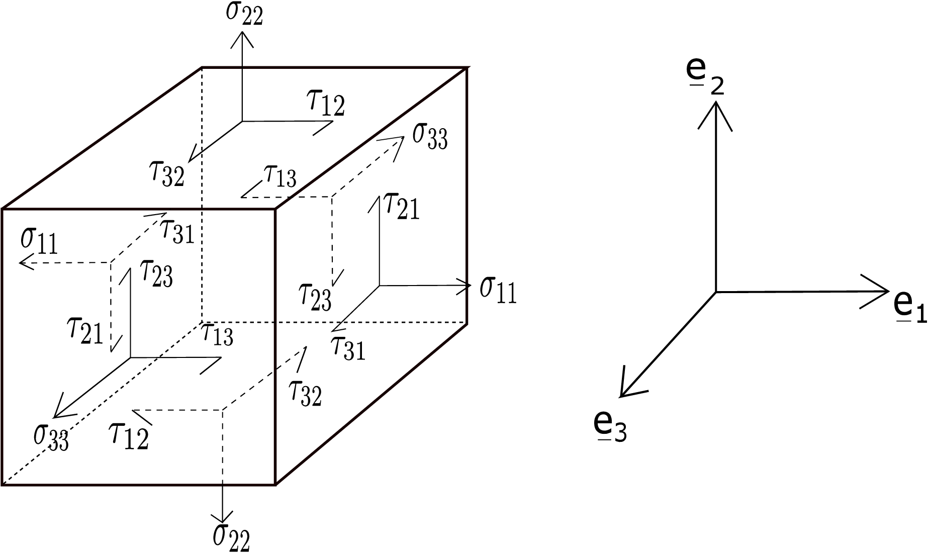
Figure 3.3: Traction components on various faces of the cuboid along with the coordinate system

We have drawn traction components on all its faces. Let us now find the moment due to these traction components about \(\underline {e}_3\) axis passing through the centroid of the cuboid. The normal components \(\sigma _{11}\), \(\sigma _{22}\) and \(\sigma _{33}\) pass through the centroid and thus do not contribute to this moment. The components \(\tau _{31}\) and \(\tau _{32}\) also do not contribute to this moment as they are parallel or anti-parallel to \(\underline {e}_3\) direction. Only contributions come from \(\tau _{12}\) and \(\tau _{21}\). The moment due to \(\tau _{21}\) will be traction times the area (\(\Delta x_2\Delta x_3\)) of the face on which it is acting times the distance of the face from the center, i.e., \(\Delta x_1/2\): it has two contributions from \(\underline {e}_1\) and \(-\underline {e}_1\) planes but both along the same direction (\(+\underline {e}_3\)). The moment due to the two \(\tau _{12}\) components acts along \(-\underline {e}_3\) direction. The moment due to body force and the contribution of rate of change of angular momentum are simply not considered in most textbooks - we have seen in our detailed derivation earlier that their contributions are of higher order. The total moment about \(\underline {e}_3\) axis (passing through the center of cuboid) will thus be

\begin {eqnarray} \left (\tau _{21}\dfrac {\Delta x_2\Delta x_3\Delta x_1}{2}\right )\times 2 -\left (\tau _{12}\dfrac {\Delta x_1\Delta x_3\Delta x_2}{2}\right )\times 2=0 ~\text {or}~\tau _{21}=\tau _{12}. \end {eqnarray}

This is a simpler derivation but it involves a strong assumption of traction components not varying on the six cuboid’s faces. Likewise, when we find the moment equation about \(\underline {e}_1\) and \(\underline {e}_2\) axis, we will get \(\tau _{23}\) = \(\tau _{32}\) and \(\tau _{13}\) = \(\tau _{31}\), respectively.

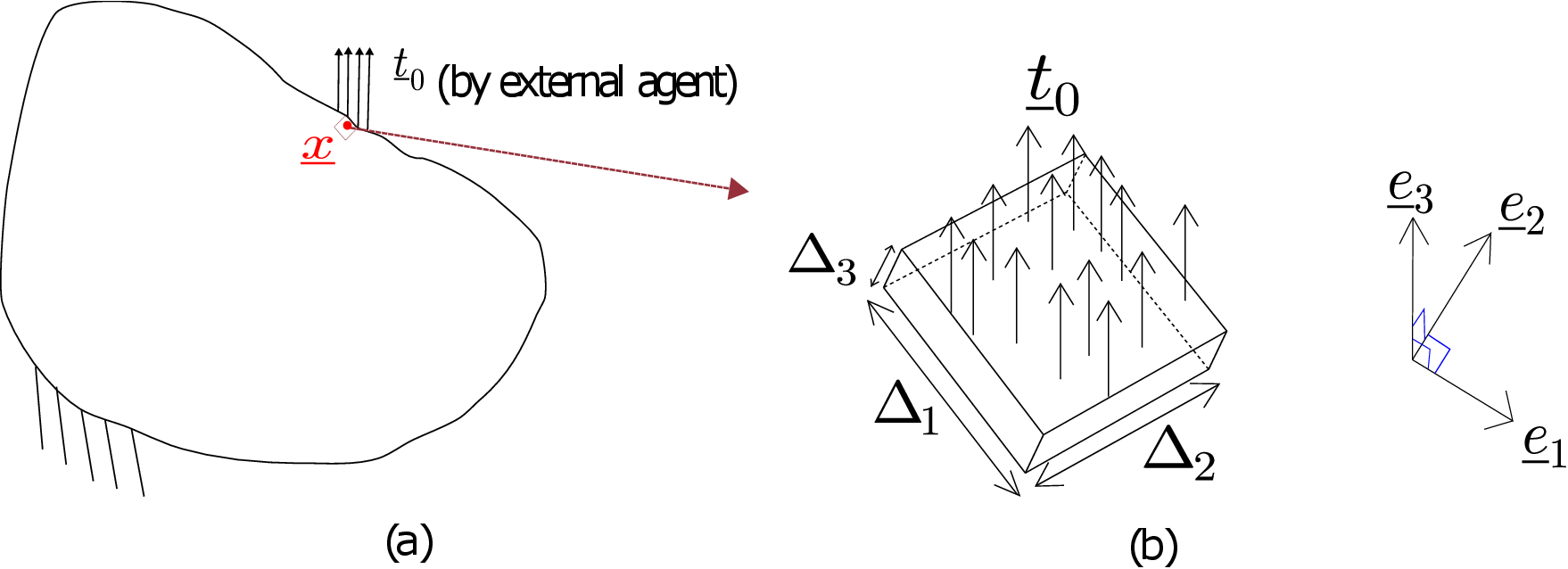
3.3 Derivation of traction boundary condition: NPTEL link

Suppose we have an arbitrary body which is clamped at some part of the boundary and a load is applied on some other part of the boundary by an external agent (see Figure 3.4a). As the applied load is usually distributed over an area, it has the unit of traction. Let us denote this applied distributed load by \(\underline {t}_0\).

Figure 3.4: (a) An arbitrary body subjected to an externally applied distributed load \(\underline {t}_0\) over its surface (b) A zoomed view of an infinitesimal part of the body close to the surface point where the external load is acting

Our aim is to find a relation between the state of stress at the point where the load is applied to the load itself. If we solve the stress equilibrium equations, we can find all the stress components everywhere in the body. However, at points on the boundary where the external load is acting, we can find the state of stress partially without solving the stress equilibrium equations. In fact, this relation that we will derive here will serve as traction boundary condition for solving stress equilibrium equations.

Let us think of an infinitesimal cuboidal part of the body near a surface point where the load is applied. Its zoomed view is shown in Figure 3.4b. Let us also set up a coordinate system such that we have \(\underline {e}_3\) axis along the local surface normal as shown in Figure 3.4b. On the top surface of this infinitesimal body part, external load \(\underline {t}_0\) is acting which we can safely assume to be acting uniformly since the body part is infinitesimal. The directions \(\underline {e}_1\) and \(\underline {e}_2\) are in the plane of the surface at that point and aligned along the edges of the infinitesimal body part. Alternatively, we can also say that these two directions are in the tangent plane at that point.^‡ So, \(\underline {e}_3\) becomes normal to this tangent plane. Let the edges of the infinitesimal body along \(\underline {e}_1, \underline {e}_2\) and \(\underline {e}_3\) directions be of lengths \(\Delta _1, \Delta _2\) and \(\Delta _3\) respectively. The total force on this infinitesimal body will be the sum of the traction forces applied from remaining part of the body, externally applied load and the body force, i.e.,

\begin {equation} \underline {t}^{-3}~ \Delta _1 \Delta _2+(\underline {t}^{2}+\underline {t}^{-2})~\Delta _1 \Delta _3+(\underline {t}^{1}+\underline {t}^{-1})~\Delta _2 \Delta _3+\underline {b}~\Delta _1 \Delta _2 \Delta _3+\underline {t}_0 ~\Delta _1 \Delta _2.\nonumber \end {equation} We now apply Newton’s \(2^{nd}\) law to this small part of the body: \begin {equation} \underline {t}^{-3} \Delta _1 \Delta _2+(\underline {t}^{2}+\underline {t}^{-2})\Delta _1 \Delta _3+(\underline {t}^{1}+\underline {t}^{-1})\Delta _2 \Delta _3+\underline {b}\Delta _1 \Delta _2 \Delta _3+\underline {t}_0 \Delta _1 \Delta _2=\rho \Delta _1\Delta _2\Delta _3~\underline {a}. \end {equation} This small body part is also called a ‘pill box’ in several textbooks. Let us divide both the sides of the above equation by \(\Delta _1 \Delta _2\) and then take the \(\lim _{\Delta _3\to 0}\), i.e.,

\begin {eqnarray} \lim _{\Delta _3 \to 0}\dfrac {\underline {t}^{-3} \Delta _1 \Delta _2+(\underline {t}^{2}+\underline {t}^{-2})\Delta _1 \Delta _3+(\underline {t}^{1}+\underline {t}^{-1})\Delta _2 \Delta _3+\underline {b}\Delta _1 \Delta _2 \Delta _3+\underline {t}_0 \Delta _1 \Delta _2}{\Delta _1 \Delta _2}&=&\dfrac {\rho \Delta _1\Delta _2\Delta _3~\underline {a}}{\Delta _1 \Delta _2}\nonumber \\ \Rightarrow \lim _{\Delta _3 \to 0}\Big [\underline {t}^{-3}+\underline {t}_0 +(\underline {t}^{2}+\underline {t}^{-2})\dfrac {\Delta _3}{\Delta _2}+(\underline {t}^{1}+\underline {t}^{-1})\dfrac {\Delta _3}{\Delta _1}+(\underline {b}-\rho \underline {a})\Delta _3&=&\underline {0}\Big ].\label {3_pillbox} \end {eqnarray}

As we take this limit, we are essentially shrinking the pill box height by pushing its bottom surface towards the top surface keeping its surface area \(\Delta _1 \Delta _2\) constant. The terms containing \(\Delta _3\) in \eqref{3_pillbox} vanish in this limit and we get \begin {equation} \underline {t}^{-3}=-\underline {t}_0. \end {equation} As \(\underline {t}^{3}\) and \(\underline {t}^{-3}\) form an action reaction pair, we finally obtain \begin {equation} \label {3_traction_to_external} \underline {t}^{3}=\underline {\underline {\sigma }}~\underline {e}_3=\underline {t}_0. \end {equation} This is the relation that we had set out to obtain. It essentially implies that the internal traction that generates in a body at its surface point and on an internal section that is parallel to local surface plane of the body is equal to the externally applied distributed load there. As mentioned earlier, this is also used as boundary condition for solving the stress equilibrium equation and is called the traction boundary condition. The above result might appear intuitive and trivial. However, we cannot directly say that \(\underline {t}_{0}=\underline {t}^{3}\) because they are two different quantities - the former is the externally applied load while the latter is the internal response of the body. We won’t be able to conclude anything about \(\underline {t}^{1}\) or \(\underline {t}^{2}\) at the surface point from this derivation though.

Relating stress matrix at surface point with external load: NPTEL link

Suppose, we want to find stress matrix at the surface point with respect to the chosen coordinate system as in Figure 3.4b. We know that the columns of stress matrix are formed by tractions on \(\underline {e}_1\), \(\underline {e}_2\) and \(\underline {e}_3\) planes. Thus, using equation \eqref{3_traction_to_external}, we know that the third column is the externally applied load per unit area. As a stress matrix has to be symmetric, its third row also becomes known to us. So, five entries of this stress matrix at surface points become known to us right away as shown below: \begin {equation} \begin {bmatrix} \underline {\underline {\sigma }} \end {bmatrix}= \begin {bmatrix} \times & \times & {t}_{0}^1\\ \times & \times & {t}_{0}^2\\ {t}_{0}^1 & {t}_{0}^2 & {t}_{0}^3\\ \end {bmatrix}. \end {equation} The remaining four entries are still unknowns (out of which only three are independent as the stress matrix has to be symmetric) and can be found only after solving the stress equilibrium equations in the entire body. As a special case, if there are parts of the boundary where no external load is being applied, i.e., \(\underline {t}_{0}\)=0, then the third row and third column of the stress matrix become zero at those boundary points.

3.4 Solved examples

Q1. A cylindrical rod is subjected to a torque T at both its ends. Its lateral surface is assumed to be traction free. We will learn later that at any point in its cross-section, the following stress components exist: \[\sigma _{xx}=\sigma _{yy}=\sigma _{zz}=\tau _{xy}=\tau _{yx}=0, \; \tau _{xz}=\tau _{zx}=-G\kappa {y},\; \tau _{yz}=\tau _{zy}=G\kappa {x}.\]

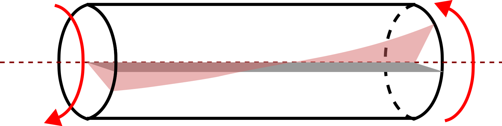
Here \(G\) is a material parameter and \(\kappa \) is the twist induced in the rod due to torque. Show that this stress distribution satisfies the governing equations of equilibrium. Does it satisfy traction free boundary condition on the rod’s lateral surface?

Solution: Let us use cylindrical coordinate system with z-axis lying along the rod’s length. Neglecting weight of the rod, the body force components become zero. Moreover, the rod is not in motion. Hence, the three acceleration components are also zero. Substituting the given values of stress components in equilibrium equations, we get \begin {align*} \dfrac {\partial \cancelto {0}{\sigma _{xx}}}{\partial x} \;+\; \dfrac {\partial \cancelto {0}{\tau _{xy}}}{\partial y}+\cancelto {0}{\dfrac {\partial \tau _{xz}}{\partial z}}\; &=\;0,\\ \dfrac {\partial \cancelto {0}{\tau _{yx}}}{\partial x} \;+\; \dfrac {\partial \cancelto {0}{\sigma _{yy}}}{\partial y}+\cancelto {0}{\dfrac {\partial \tau _{yz}}{\partial z}}\; &=\;0,\\ \cancelto {0}{\dfrac {\partial \tau _{zx}}{\partial x}} \;+\; \cancelto {0}{\dfrac {\partial \tau _{zy}}{\partial y}}+ \dfrac {\partial \cancelto {0}{\sigma _{zz}}}{\partial z}\; &=\;0 . \end {align*}

Hence, the three equations are satisfied. To show that the lateral surface is free of external load, we apply the relation of traction boundary condition with the external load. The unit outward normal on the lateral surface is perpendicular to z-axis, i.e.,

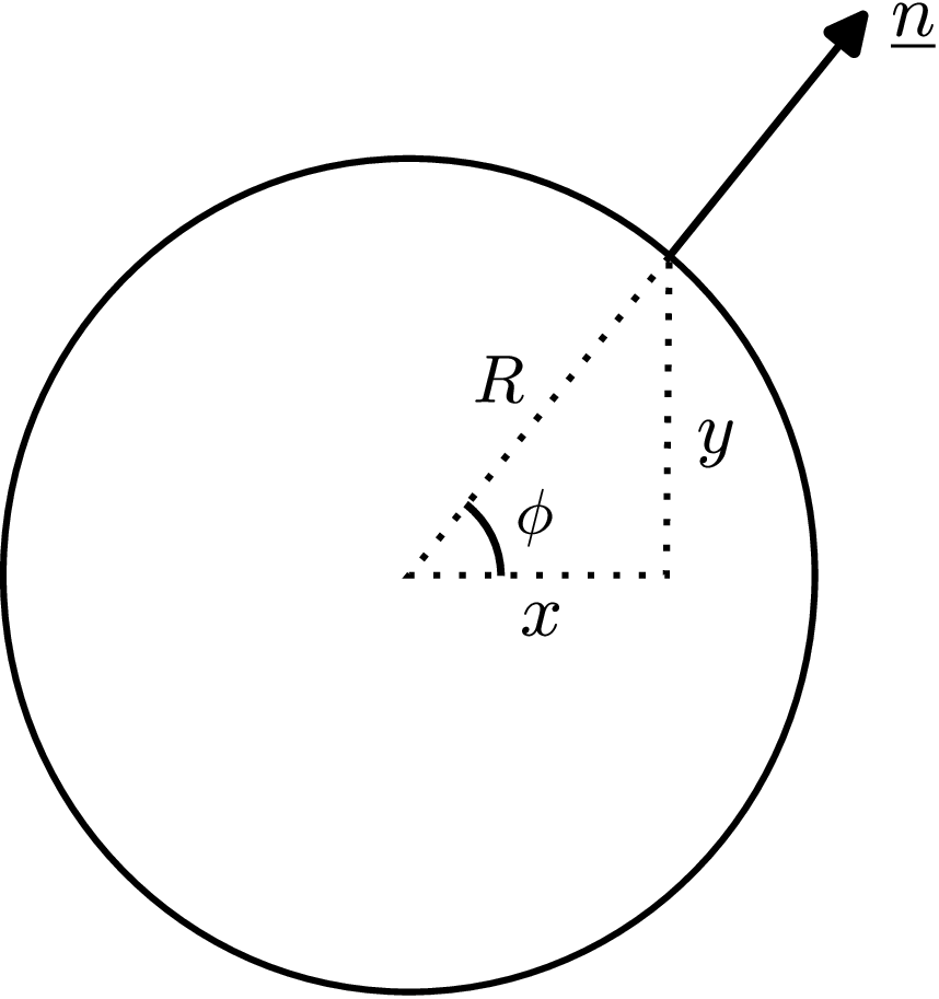
\begin {align*} \sbk {\ve {n}} = \begin {bmatrix} \cos \phi \\ \sin \phi \\ 0 \end {bmatrix} = \begin {bmatrix} x/R \\ y/R \\ 0 \end {bmatrix}\Rightarrow \sbk {\ve {t}^n} = \sbk {\matr {\sigma }} \sbk {\ve {n}} ~~= \begin {bmatrix} 0 & 0 & -G \theta y \\ 0 & 0 & \phantom {-} G \theta x \\ -G \theta y & G \theta x & 0 \end {bmatrix} \begin {bmatrix} x/R \\ y/R \\ 0 \end {bmatrix} = \begin {bmatrix} 0 \\ 0 \\ 0 \end {bmatrix}. \end {align*}

For an exhaustive set of solved examples and unsolved objective and subjective type questions, please refer to the printed book.

^∗If we do balance of angular momentum about a moving point, we get an extra term in the equation.

^†Just like linear momentum balance, angular momentum balance is also applied always to a fixed/identifiable mass. If we choose our system to be a fixed cuboidal volume in space, the mass contained in the cuboid will change with time since mass is transporting through its surfaces and hence we cannot apply linear or angular momentum balance to it.

^‡The tangent plane to a curved surface is a plane that just touches the surface locally.

[next] [prev] [prev-tail] [front] [up]

Chapter 3Stress Equilibrium Equations