In this chapter, we will learn about the concept of traction vector, stress tensor and its matrix representation. We will also learn how to transform stress matrix corresponding to one coordinate system into another.
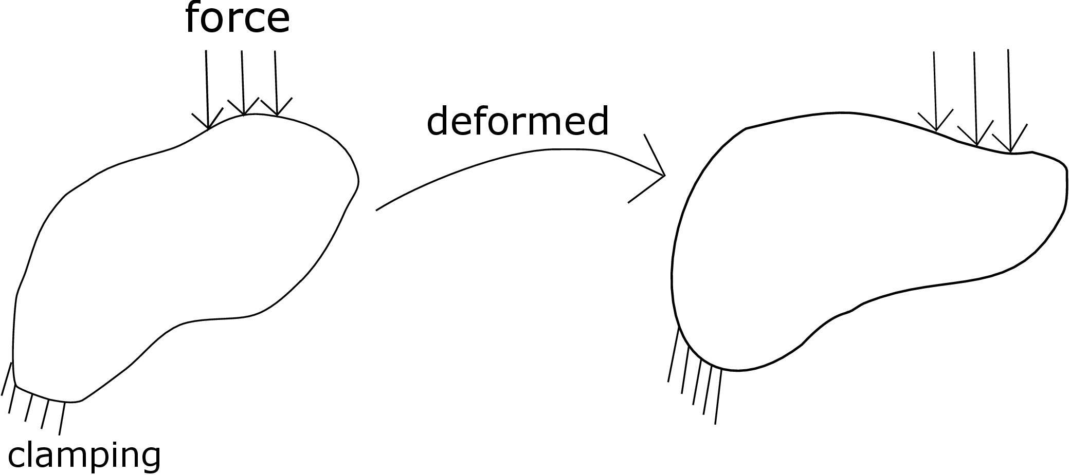
Consider an arbitrary body which is clamped at one part of the boundary and some external load is applied elsewhere on its boundary (see Figure 2.1). The clamped boundary of the body does not move but the remaining body deforms due to the applied load.
In the deformed state, we say that the body is under some stress. Let us imagine cutting the deformed body into two parts A and B through an internal section as shown by the dashed lines in Figure 2.2.
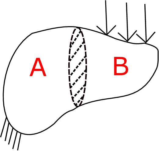
Let us analyze part A. The part B exerts some force on part A through the internal section - this force is distributed over the internal section as shown in Figure 2.3a.
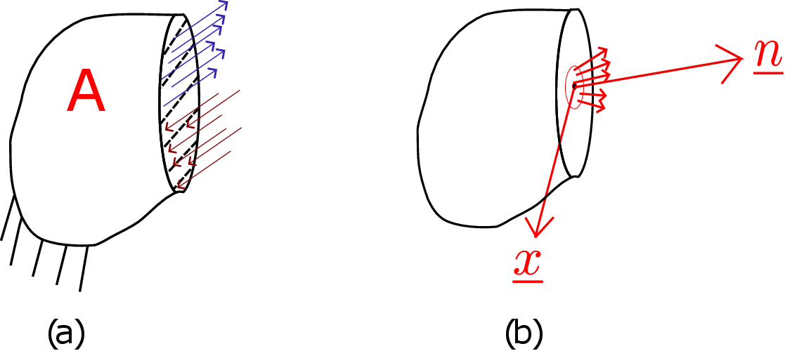
We define traction to be the intensity of the force (force per unit area) with which Part B is pulling or pushing part A. At different points in the section, this force intensity would be different in both magnitude and direction. For example, the upper portion of the section is being pulled while the bottom portion is being pushed. To find traction at some point \(\underline {x}\) on the section (see Figure 2.3b), we draw a circle around this point in the plane of the section. Let the area enclosed by the circle be \(\Delta A\) and the net force acting on this circular area be \(\Delta \overrightarrow F\). We then shrink the area of the circle such that the circle always contains \(\underline {x}\). As we shrink the area, the total force acting on it decreases but the ratio of this force and the area of the enclosing circle attains a limiting value which is called traction. We represent it by \(\underline {t}(\underline {x};\underline {n})\) where \(\underline {n}\) denotes the normal to the section but pointing outward/away from part A on which it is acting. Mathematically, we write \begin {equation} \underline {t}(\underline {x};\underline {n})=\lim _{\Delta A \to 0} \frac {\Delta \overrightarrow F}{\Delta A}. \end {equation} Although it has the unit of pressure, it is more general than pressure: pressure always acts in the direction opposite to the outward plane normal whereas traction can act in an arbitrary direction.
Think of an arbitrary body under the influence of external load and consider three points inside it (see Figure 2.4).
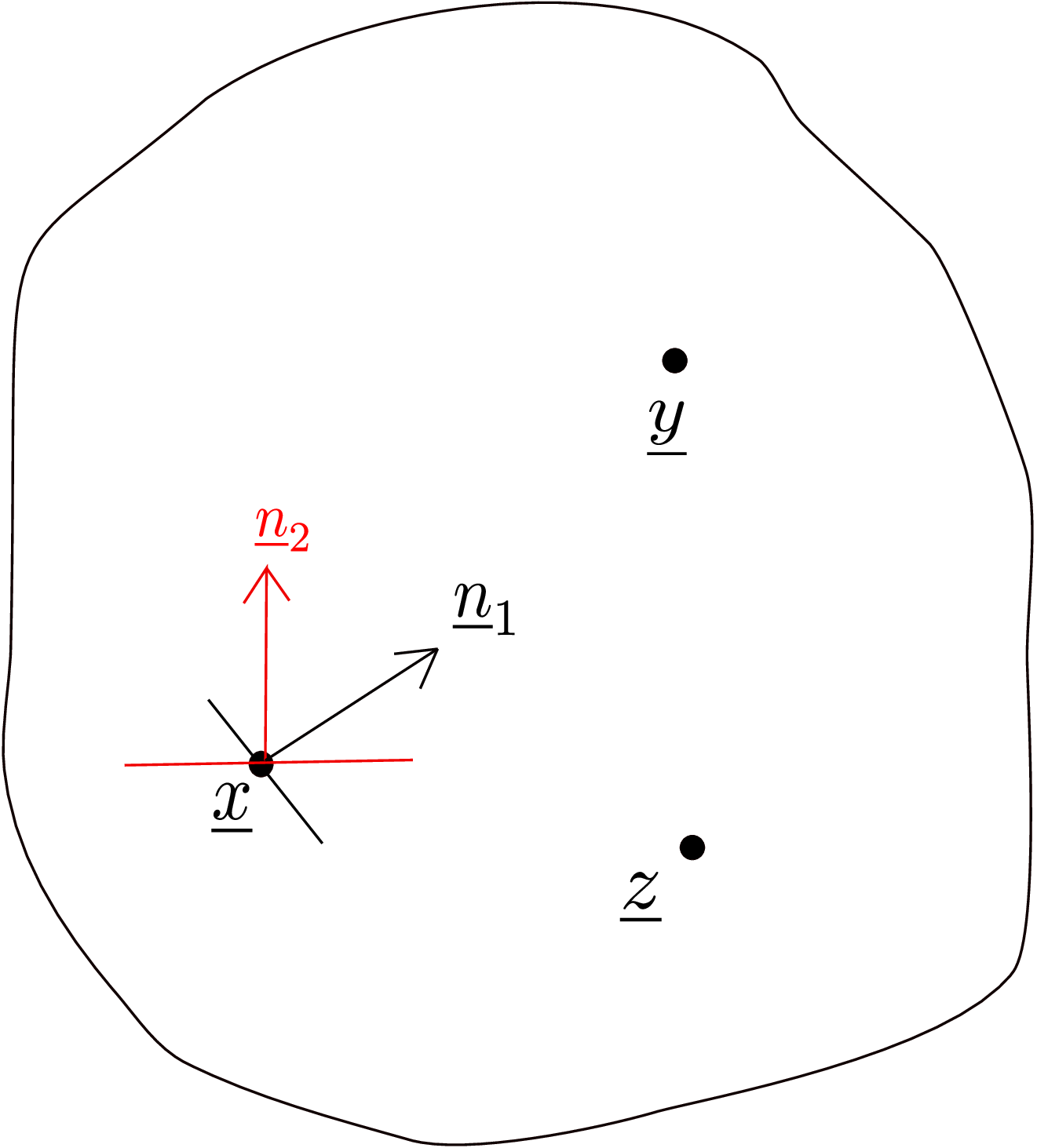
In general, traction will be different at these three points. At a given point also, say \(\underline {x}\), several planes/internal sections can be imagined and traction on each of these planes will be different. In Figure 2.4 for example, traction on the plane having normal \(\underline {n}_1\) will be different from traction on plane having normal \(\underline {n}_2\). To see this more clearly, let us consider a rectangular beam which is clamped at one end (see Figure 2.5). A force P is being applied to its other end. The cross-sectional area of the beam is \(A\). From force balance of the entire beam, we can show that the clamped support at the left end exerts a force \(-P\underline {e}_1\) to the leftmost end of the beam.
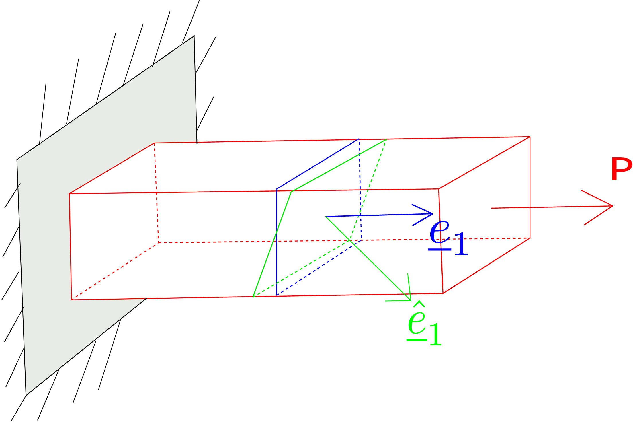
Let us now consider an internal section of the beam whose normal vector (denoted by \(\underline {e}_1\)) is along the axis of the beam (also shown as the blue plane in Figure 2.5). This section divides the beam into two parts. From the force balance of left portion of the beam, one can show that the total internal force on this section also equals \(P\underline {e}_1\). Hence, the traction on this plane (denoted by \(\underline {t}^1\)) is given by \begin {equation} \underline {t}^1=\frac {P\underline {e}_1}{A}=\frac {P}{A}~\underline {e}_1. \end {equation} Notice that traction is acting along the plane normal only and hence we call it the normal traction.∗ Now, let us take an inclined internal section (shown in green in Figure 2.5) but at the same axial location as the vertical plane. The unit normal to this new section (\(\underline {\hat e}_1\)) makes an angle \(\theta \) with the beam’s axis. So, the area of this section \(\hat A\) is given by \begin {equation} \hat A=\frac {A}{\cos \theta }. \end {equation} From force balance of the new left portion of the beam, one can show that the total force on the new inclined/green section is still P\(\underline {e}_1\). So, the traction on this section (denoted by \(\underline {t}^{\hat 1}\)) will be \begin {equation} \underline {t}^{\hat 1}=\frac {P\underline {e}_1}{A/\cos \theta }=\frac {P\cos \theta }{A}\underline {e}_1 \end {equation} Thus, we see that traction on two different planes at the same point are different. Also note that the traction vector now is not aligned with the plane normal. Its component along the plane normal is called the normal component of traction and equals \(\frac {P}{A}\cos ^2\theta \) in this case. On the other hand, the component of traction perpendicular to the plane normal is called the shear component of traction and equals \(\frac {P}{A}\cos \theta \sin \theta \). Note that the shear component becomes maximum for the section for which \(\theta =45^{\circ }\).
By definition, it gives us the intensity of force with which one part of the body is pulling or pushing the other part of the body. If the value of this traction is lower than a threshold limit, the body will not fracture/fail. At a given point, as traction varies from one plane to the other, the probability of failure is higher on the plane on which traction has got larger value. Thus, traction can tell us at what point in the body and on what plane at that point would the body fail! For example, it has been experimentally observed during tensile loading of a steel bar that at a critical value of applied load, the steel bar develops a crack in a plane that is inclined at around \(45^{\circ }\) to the direction of loading. This is because on this plane, the magnitude of shear component of traction is highest as we saw earlier. We clarify at this point that failure due to shear component of traction reaching a critical value is just one mechanism of failure and different materials obey different mechanisms of failure.
We will now prove that if we know traction on three mutually perpendicular planes at a point, we can find traction on any plane at that point. Let us consider a point \(\underline {x}\) in the body as shown in Figure 2.6 and imagine a small volume there in the shape of a tetrahedron with its vertex at \(\underline {x}\). The tetrahedron’s three edges at this point are assumed to be perpendicular to each other and lying along the three coordinate axes.
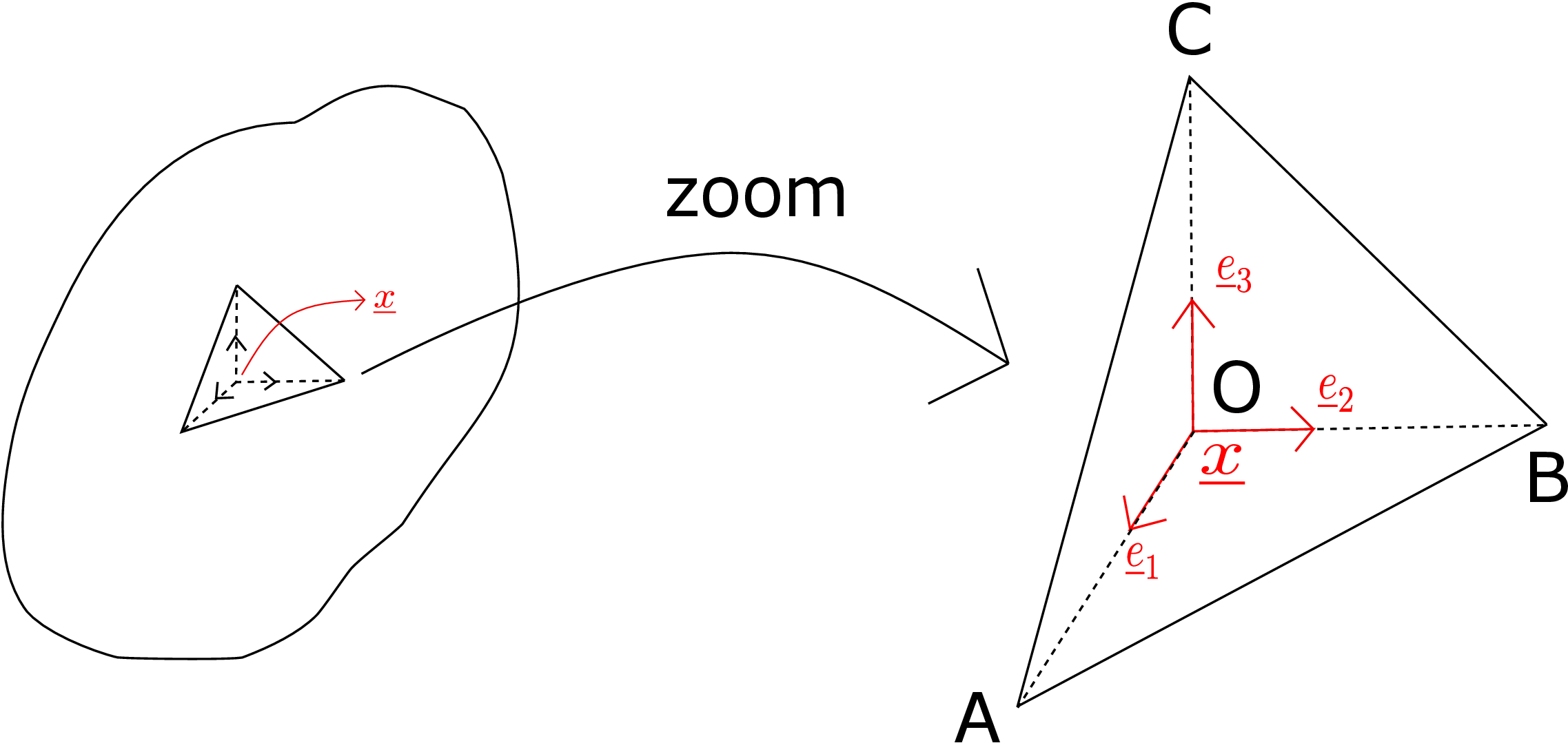
This tetrahedron has four faces having the following outward normals (by outward we mean pointing out of the tetrahedron volume):
Suppose, we know traction on three of these planes having outward normals (\(-\underline {e}_1, -\underline {e}_2,-\underline {e}_3\)) and we want to find traction on the tilted plane ABC (having normal say \(\underline {n}\)). Let us apply Newton’s \(2^{nd}\) law of motion to the mass contained in the tetrahedron: \begin {equation} \sum \underline {F}^{ext}= \frac {d}{dt}(\overrightarrow {P}). \end {equation} Here \(\overrightarrow {P}\) denotes the linear momentum of the tetrahedron’s mass. To visualize the external forces acting on the tetrahedron, we can imagine taking out the tetrahedron from the original body as shown on the right of Figure 2.6. The remaining part of the body exerts traction force on the four faces of the tetrahedron which are also categorized as surface force. However, the total external force consists of both surface and body forces: \begin {equation*} \sum \underline {F}^{ext} \end {equation*} \begin {equation*} \swarrow \hspace {15mm}\searrow \end {equation*} \begin {equation*} (surface\hspace {2mm}force)\hspace {15mm}(body\hspace {2mm}force) \end {equation*} \begin {equation*} \text {unit: [force/area]}\hspace {20mm}\text {unit: [force/volume]} \end {equation*} The body force acts on every point of the body, e.g., the gravitational force is applied by the Earth on every point of the tetrahedron. Its unit is force/volume as it acts on the entire volume in a distributed manner and is given by \begin {equation} \text {Gravitational body force}=(\rho \underline {g} V)/V=\rho \underline {g}. \end {equation} Here \(\rho \) denotes density, \(\underline {g}\) is acceleration due to gravity and \(V\) is volume of the tetrahedron. To obtain the total surface force, we need to integrate traction forces over the area on which they are acting whereas to get the total body force, we need to integrate body force over the volume of the tetrahedron. Let the area of face OBC be \(A_1\) and traction on it be \(\underline {t}^{-1}\), area of face OAC be \(A_2\) and traction on it be \(\underline {t}^{-2}\), area of face OAB be \(A_3\) and traction on it be \(\underline {t}^{-3}\) and finally the area of face ABC be \(A_n\) and traction on it be \(\underline {t}^{n}\). The total external force on the tetrahedron can be written as \begin {equation} \label {2_total_force} \sum \underline {F}^{ext}=\underbrace {\underline {t}^{-1}_{avg} A_1+ \underline {t}^{-2}_{avg} A_2+\underline {t}^{-3}_{avg} A_3+ \underline {t}^{n}_{avg} A_n}_{\text {contact force}}+\underbrace {\rho \underline {g}V}_{\text {non-contact force}}=\underbrace {\rho V}_{\text {tetrahedron mass}}\times ~\underline {a}_{CM}. \end {equation} Here \(\underline {a}_{CM}\) denotes the acceleration of center of mass of the tetrahedron. The subscript “avg” on four tractions is used to denote that they are the average values of traction on corresponding faces. Suppose \(h\) is the perpendicular distance of the plane ABC from the tetrahedron’s vertex. The volume of the tetrahedron is then given by \begin {equation} \label {2_Volume} V=\frac {A_n h}{3}. \end {equation} We can also relate the areas \(A_ 1\), \(A_2\), \(A_ 3\) in terms of \(A_n\). If we project the area \(A_ n\) along the direction \(\underline {e}_ 1\), it will turn out to be the same as the area of OBC which is \(A_1\). We can thus write \begin {equation} \label {2_projection_area} A_i=A_n(\underline {n}\cdot \underline {e}_i)~\forall i=1,2,3. \end {equation} Upon plugging equations \eqref{2_Volume} and \eqref{2_projection_area} into equation \eqref{2_total_force}, we then get \begin {equation*} A_n\left (\underline {t}^{-1}_{avg}(\underline {n}\cdot \underline {e}_1)+\underline {t}^{-2}_{avg}(\underline {n}\cdot \underline {e}_2)+\underline {t}^{-3}_{avg}(\underline {n}\cdot \underline {e}_3)+\underline {t}^{n}_{avg}\right ) + \frac {\rho \underline {g} A_n h}{3} = \frac {\rho A_n h~ \underline {a}_{CM}}{3} \end {equation*} \begin {equation} \label {2_traction_before_limit} \Rightarrow \underline {t}^{n}_{avg}+\sum _{i=1}^3 \underline {t}^{-i}_{avg}(\underline {n} \cdot \underline {e}_i)+\frac {\rho h (\underline {g}-\underline {a}_{CM})}{3}=0. \end {equation} Here we obtained the last equation upon dividing by the tilted area \(A_n\). Note that our original plan was to obtain traction on an arbitrary plane \(\underline {n}\) at a point in terms of traction on three other planes at the same point. However, for our tetrahedron example, three planes pass through the point O but the plane with normal \(\underline {n}\) (the tilted plane) does not pass through the point O. So, we need to shrink the tetrahedron such that in the limiting case, all the four planes pass through O. We can achieve this by letting the perpendicular distance \(h\) go to zero. When we apply this limit (\(\lim _{h\to 0}\)) to equation \eqref{2_traction_before_limit}, the terms proportional to \(h\) vanish. Furthermore, the average tractions become the corresponding traction values at the point \(\underline {x}\) itself. Thus, in the limit of tetrahedron shrinking to point \(\underline {x}\) where all the four planes exist now, the terms corresponding to body force and acceleration vanish and we get the following desired result: \begin {equation} \label {2_traction_after_limit} \underline {t}^n(\underline {x}) =-\sum _{i=1}^3 \underline {t}^{-i}(\underline {x})~(\underline {n}\cdot \underline {e}_i). \end {equation}
By definition, \(\underline {t}^{-i}\) is the traction on \(-\underline {e}_{i}\) plane whereas \(\underline {t}^{i}\) is the traction on \(\underline {e}_{i}\) plane. The two tractions basically act on the same plane but with normals pointing in opposite direction. Let us understand it in the context of an internal section in the body from Figure 2.2. We redraw the two parts so created in Figure 2.7.
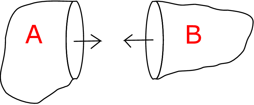
The original internal section now forms external surface of the two parts of the body and have outward normals pointing opposite to each other.† The tractions on these two planes (the two planes were coincident in the original body) will be equal and opposite due to Newton’s third law since they form action-reaction pair. We can thus write \begin {equation} \label {traction_opposite_planes} \underline {t}^{-i}=-\underline {t}^{i}. \end {equation} Substituting it in equation \eqref{2_traction_after_limit}, we finally obtain \begin {equation} \boxed {\underline {t}^n(\underline {x}) =\sum _{i=1}^3 \underline {t}^{i}(\underline {x})~(\underline {n}\cdot \underline {e}_i)} \end {equation} We emphasize that the body force and acceleration terms dropped out from the above formula - no approximation was made! Thus, the above formula holds even if the body force is present or the body is accelerating! Physically, the traction vector \(\underline {t}^n\) has to be the same irrespective of what three planes are used to find it, i.e., \begin {equation} \label {2_traction_two_coordinate_systems} \underline {t}^n(\underline {x}) =\sum _{i=1}^3 \underline {t}^{i}(\underline {x})~(\underline {n}\cdot \underline {e}_i) =\sum _{i=1}^3 \underline {t}^{\hat i}(\underline {x}) ~(\underline {n}\cdot \underline {\hat e}_i ). \end {equation} In the first case, the three planes used have normals along \(\underline {e}_1\), \(\underline {e}_2\), \(\underline {e}_3\) whereas in the second case, the three planes have normals along \(\underline {\hat e}_1\), \(\underline {\hat e}_2\), \(\underline {\hat e}_3\).
Let us now write equation \eqref{2_traction_two_coordinate_systems} in a slightly different way: \begin {equation} \label {2_traction_arbitrary_plane} \underline {t}^n(\underline {x}) =\sum _{i=1}^3\underline {t}^{i}(\underline {x})~(\underline {n}\cdot \underline {e}_i)=\sum _{i=1}^3\underline {t}^{i}(\underline {x})~(\underline {e}_i \cdot \underline {n}). \end {equation} The \(i\)th term in the above summation can be written as follows in matrix form: \begin {equation} \Bigg [\hspace {3mm}\Bigg ]_{3\times 1}\Bigg ([\hspace {7mm}]_{1\times 3}\Bigg [\hspace {3mm}\Bigg ]_{3\times 1}\Bigg ) \end {equation} \begin {equation*} \downarrow \hspace {15mm}\downarrow \hspace {12mm}\downarrow \hspace {7mm} \end {equation*} \begin {equation*} \underline {t}^i\hspace {15mm}\underline {e}_i^T\hspace {12mm}\underline {n}\hspace {7mm} \end {equation*} As matrix multiplication is associative, we can also write it alternatively as \begin {equation} \label {2_rearrangement} \Bigg (\Bigg [\hspace {3mm}\Bigg ]_{3\times 1}[\hspace {7mm}]_{1\times 3}\Bigg )\Bigg [\hspace {3mm}\Bigg ]_{3\times 1} \end {equation} \begin {equation*} \downarrow \hspace {12mm}\downarrow \hspace {14mm}\downarrow \end {equation*} \begin {equation*} \underbrace {\underline {t}^i\hspace {12mm}\underline {e}_i^T}_{\text {tensor product}}\hspace {14mm}\underline {n} \end {equation*} However, note that \([\underline {a}][\underline {b}]^T\) is the matrix representation for tensor product (\(\underline {a}\otimes \underline {b}\)). Thus, the alternate representation given by \eqref{2_rearrangement} can be written as follows in tensor form: \begin {equation} \label {final_traction} \underline {t}^n(\underline {x})=\underbrace {\sum _{i=1}^3(\underline {t}^{i}(\underline {x}) \otimes \underline {e}_i)}_{\text {stress tensor}}\cdot ~\underline {n}. \end {equation} This is just a different viewpoint but the interesting point here is that the orientation \(\underline {n}\) has been separated. One could have also obtained it directly from equation \eqref{2_traction_arbitrary_plane} using the definition of dot product of a second order tensor with a vector. The tensor that is multiplied with \(\underline {n}\) in the above expression is called the stress tensor \(\underline {\underline {\sigma }}\) and one can write \begin {equation} \label {2_stress_tensor_definition} \underline {\underline {\sigma }}(\underline {x})=\sum _{i=1}^3 \underline {t}^{i}(\underline {x}) \otimes \underline {e}_i~\text {such that}~ \underline {t}^n(\underline {x})=\underline {\underline {\sigma }}(\underline {x})~\underline {n}. \end {equation} Note that the stress tensor depends on \(\underline {x}\) alone. Essentially, to obtain the stress tensor at a point, choose three independent planes at that point, find tractions on those planes, do their tensor product with corresponding plane normals and sum! The resulting stress tensor will be independent of what specific set of three planes we choose!
Let us try to represent equation \eqref{2_stress_tensor_definition} in (\(\underline {e}_1\), \(\underline {e}_2\), \(\underline {e}_3\)) coordinate system. As we now know that the stress tensor is a second order tensor, its representation is going to be a matrix, i.e., \begin {equation*} \begin {bmatrix} \underline {\underline {\sigma }} \end {bmatrix}_{(\underline {e}_1,\underline {e}_2,\underline {e}_3)}= \sum _{i=1}^3 \begin {bmatrix} \underline {t}^i \end {bmatrix} \begin {bmatrix} \underline {e}_i \end {bmatrix}^T. \end {equation*} Here we have to represent \(\underline {t}^i\) and \(\underline {e}_i\) both in \((\underline {e}_1,\underline {e}_2,\underline {e}_3)\) coordinate system, i.e.,
Here \(t_j^i=\underline {t}^i\cdot \underline {e}_j\) represents the \(j^{th}\) component of traction on \(i^{th}\) plane. Thus, if we want to write the stress matrix corresponding to (\(\underline {e}_1\),\(\underline {e}_2\),\(\underline {e}_3\)) coordinate system, its first column would be the representation of traction on plane whose normal is along the first coordinate axis (which is \(\underline {e}_1\) here). Similarly, the second column will be the representation of traction on plane with normal along second coordinate axis and the third column will be the representation of traction on plane with normal along third coordinate axis. It is important to obtain the representation/ column form of the three tractions also in the same coordinate system. Usually, the following notation is used to write the stress matrix: \begin {equation} \label {stressmatrix} \begin {bmatrix} \underline {\underline {\sigma }} \end {bmatrix}_{(\underline {e}_1,\underline {e}_2,\underline {e}_3)}= \begin {bmatrix} \sigma _{11} & \tau _{12} & \tau _{13}\\ \tau _{21} & \sigma _{22} & \tau _{23} \\ \tau _{31} & \tau _{32} & \sigma _{33}\\ \end {bmatrix}. \end {equation} Basically, the off-diagonal elements denote shear components of traction and are denoted by \(\tau \) whereas diagonal components denote normal components of traction and are denoted by \(\sigma \). On comparing the above form with \eqref{2_stresscomponentrepresentation}, \(\tau _{ij}\) denotes the \(i^{th}\) component of traction on \(j^{th}\) plane.‡
Let us say we want to represent the stress tensor at a given point \(\underline {x}\) in our body.
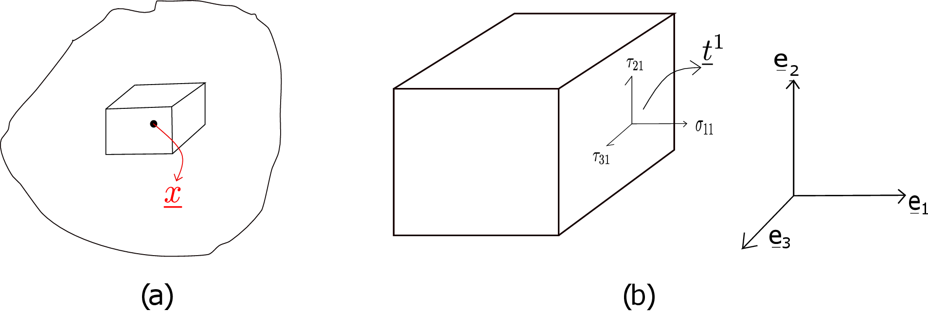
Think of a cuboid around point \(\underline {x}\) with its center at \(\underline {x}\) and its six faces chosen along \(\underline {e}_1\), \(\underline {e}_2\), \(\underline {e}_3\), -\(\underline {e}_1\), -\(\underline {e}_2\) and -\(\underline {e}_3\) (see Figure 2.8). The traction that acts on its \(\underline {e}_1\) face is \(\underline {t}^1\) whose three components are shown in Figure 2.8b. From the figure, it can be concluded that \(\sigma _{11}\) acts normal to the plane whereas \(\tau _{21}\) and \(\tau _{31}\) are in the plane. Thus, \(\sigma _{11}\) is the normal component of traction and \(\tau _{21}\) and \(\tau _{31}\) are the shear components of traction since they try to shear the body. To visualize shear, think of an internal section in the body. If the traction on this section has a non-zero component in the plane of the section, then the parts of the body on the two sides of the section will try to shear relative to each other, i.e., relatively displace along the plane of the section itself. Similarly, normal component of traction will lead to pushing or pulling between the two parts. If it is positive (negative), we call it tensile (compressive) since the two parts will try to pull (push) themselves apart (into each other). Going back to our cuboid, the components of traction that acts on all its faces are shown in Figure 2.9. Remember that the second index denotes plane normal whereas the first index denotes direction.
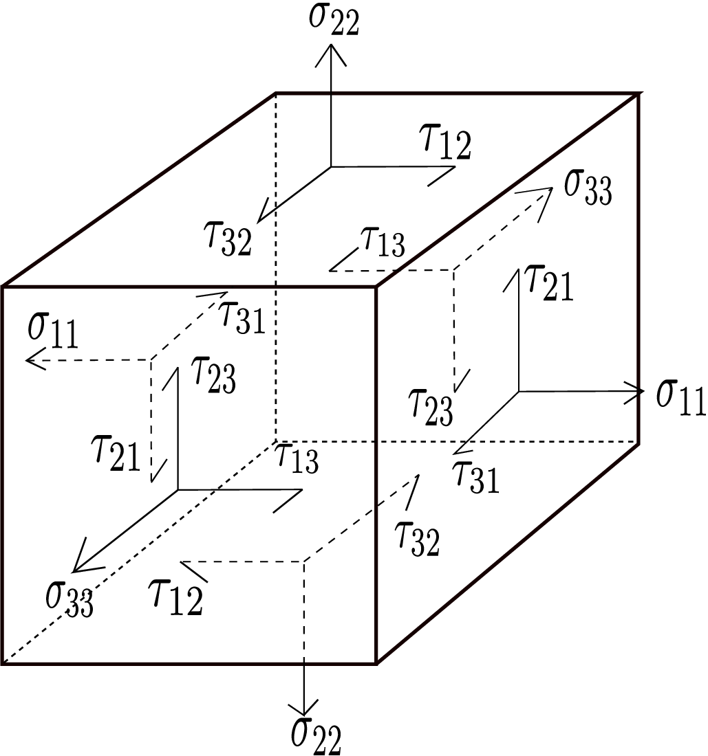
For faces with negative normals such as the bottom face, the plane normal is along -\(\underline {e}_2\) and hence \(\underline {t}^{-2}\) acts on it. We have already seen in the last lecture that \begin {equation} \underline {t}^{-2}=-\underline {t}^2. \end {equation} So, the same traction components that act on the top face also act on the bottom face but directed oppositely. In fact, as per convention, a positive value for traction component implies that it acts along positive direction on positive planes but along negative direction on negative planes. Finally, if the various components drawn on the cuboid have to represent the components of stress matrix at a point \(\underline {x}\) in the body, the cuboid must be shrunk to this point and made infinitesimally small so that all its faces pass through \(\underline {x}\). In the above figures however, we have drawn the cuboid bigger and the point \(\underline {x}\) at the center of the cuboid for better visualization.
We have learnt that stress matrix is the representation (matrix form) of stress tensor in a coordinate system. It changes from one coordinate system to another but the stress tensor itself remains unchanged. The goal here is to obtain a relationship between stress matrices in two different coordinate systems. The stress matrix in (\(\underline {e}_1\),\(\underline {e}_2\),\(\underline {e}_3\)) coordinate system is \begin {equation*} \hspace {12mm}\begin {bmatrix} \underline {\underline {\sigma }} \end {bmatrix}_{(\underline {e}_1,\underline {e}_2,\underline {e}_3)}= \Bigg [\Bigg (\hspace {2mm}\Bigg )\Bigg (\hspace {2mm}\Bigg )\Bigg (\hspace {2mm}\Bigg )\Bigg ]~\text {such that}~\sigma _{ij}=\underline {t}^j\cdot \underline {e}_i. \end {equation*} \begin {equation*} \downarrow \hspace {7mm}\downarrow \hspace {7mm}\downarrow \end {equation*} \begin {equation*} [\underline {t}^1]\hspace {5mm}[\underline {t}^2]\hspace {5mm}[\underline {t}^3] \end {equation*} Similarly, writing down the stress matrix in a new coordinate system (\(\underline {\hat e}_1,\underline {\hat e}_2,\underline {\hat e}_3\)), we get \begin {equation*} \hspace {30mm}\begin {bmatrix} \underline {\underline {\sigma }} \end {bmatrix}_{(\underline {\hat e}_1,\underline {\hat e}_2,\underline {\hat e}_3)}= \Bigg [\Bigg (\hspace {2mm}\Bigg )\Bigg (\hspace {2mm}\Bigg )\Bigg (\hspace {2mm}\Bigg )\Bigg ]~\text {such that}~\hat \sigma _{ij}=\underline {t}^{\hat j}\cdot \underline {\hat e}_i~(\neq \underline {t}^{\hat j}\cdot \underline {e}_i). \end {equation*} \begin {equation*} \downarrow \hspace {7mm}\downarrow \hspace {7mm}\downarrow \end {equation*} \begin {equation*} [\underline {t}^{\hat 1}]\hspace {3mm}[\underline {t}^{\hat 2}]\hspace {3mm}[\underline {t}^{\hat 3}] \end {equation*} Using the above definition of \(\hat \sigma _{ij}\), we can write
Now, we need to define a relationship between (\(\underline {\hat e}_1\), \(\underline {\hat e}_2\), \(\underline {\hat e}_3\)) and (\(\underline {e}_1\), \(\underline {e}_2\), \(\underline {e}_3\)). Let us think of the rotation tensor \(\underline {\underline {R}}\) that relates one set of basis vectors to another set of basis vectors, i.e., \begin {equation} \label {2_basis_transformation} \underline {\hat e}_i=\underline {\underline {R}}\hspace {1mm}\underline {e}_i. \end {equation} The matrix form of the above rotation tensor in (\(\underline {e}_1,~ \underline {e}_2,~ \underline {e}_3\)) coordinate system, i.e., \( \begin {bmatrix} \underline {\underline {R}} \end {bmatrix}_{(\underline {e}_1, ~\underline {e}_2,~ \underline {e}_3)}\) will have its components defined by \begin {equation} \label {rotation_component} R_{ij}=(\underline {\underline {R}}\underline {e}_j)\cdot \underline {e}_i=\underline {\hat e}_j\cdot \underline {e}_i. \end {equation} Substituting it in equation \eqref{2_stress_basic}, we get
Now, by definition, \(t_m^k=\sigma _{mk}\) because \(t_m^k\) represents the \(m^{th}\) component of traction \(\underline {t}^k\) and will thus represent the \(m^{th}\) row in the \(k^{th}\) column of stress matrix. Hence \begin {equation} \hat \sigma _{ij}=\sum _k\sum _m \sigma _{mk} R_{mi} R_{kj}=\sum _k\sum _m R_{im}^T\sigma _{mk} R_{kj}. \end {equation} Finally, writing this equation in a matrix form, we get \begin {equation} \label {2_stress_transformation} \begin {bmatrix} \underline {\underline {\sigma }} \end {bmatrix}_{(\underline {\hat e}_1, ~\underline {\hat e}_2, ~\underline {\hat e}_3)}= \underbrace { \begin {bmatrix} \underline {\underline {R}} \end {bmatrix}^T \begin {bmatrix} \underline {\underline {\sigma }} \end {bmatrix} \begin {bmatrix} \underline {\underline {R}} \end {bmatrix}}_{(\underline {e}_1, ~\underline {e}_2, ~\underline {e}_3)}. \end {equation} This is the relation that we can use to transform a stress matrix from one coordinate system to another. In fact, the above relation holds for the transformation of matrix form of any second order tensor. One can use similar procedure to also relate the column form of a vector in two different coordinate systems. For example, one can deduce that \begin {equation} \begin {bmatrix} \hat v_1\\ \hat v_2\\ \hat v_3 \end {bmatrix}= \begin {bmatrix} \underline {\underline {R}} \end {bmatrix}^T_{(\underline {e}_1,~ \underline {e}_2, ~\underline {e}_3)} \begin {bmatrix} v_1\\ v_2\\ v_3 \end {bmatrix}. \end {equation} What is to be noticed here is that for transforming the vector components, we need to premultiply by \(\begin {bmatrix} \underline {\underline {R}} \end {bmatrix}^T\) whereas for relating basis vectors, we need to premultiply by \(\underline {\underline {R}}\) (see equation \eqref{2_basis_transformation}). This is because the vector \(\underline {v}\) has to remain the same, we are just trying to write it in two different coordinate systems, i.e., \begin {equation} \underline {v}=\sum v_i ~\underline {e}_i=\sum {\hat v}_i ~\underline {\hat e}_i. \end {equation} Therefore, if the basis vector gets transformed with rotation \(\underline {\underline {R}}\), the components would have to get transformed with \(\begin {bmatrix}\underline {\underline {R}}\end {bmatrix}^T\). Only then, \(\underline {\underline {R}}^T\underline {\underline {R}}\) gets cancelled with each other to become \(\underline {\underline {I}}\).
Q1. Show that \(\ve {t}^n = \msum {i} \ve {t}^{i} \brc {\ve {n} \cdot \ve {e}_i} = \msum {i} \ve {t}^{\hat {i}} \brc { \ve {n} \cdot \hat {\ve {e}}_i }\), i.e, the formula is independent of what three planes are chosen to determine \(\ve {t}^n\)!
Solution: Think of \(\brc {\ve {e}_{1}, \ve {e}_{2}, \ve {e}_{3}}\) and \( \brc {\hat {\ve {e}}_{1}, \hat {\ve {e}}_{2}, \hat {\ve {e}}_{3}}\) system which form the plane normals in the two cases. Let us expand the vector \(\ve {e}_1\) in \( \brc {\hat {\ve {e}}_{1}, \hat {\ve {e}}_{2}, \hat {\ve {e}}_{3}}\) basis, i.e., \(\ve {e}_1 = \msum {i=1}^3 \brc {\ve {e}_1\cdot \hat {\ve {e}}_i}\hat {\ve {e}}_i\). Here \(\brc {\ve {e}_1 \cdot \hat {\ve {e}}_i}\) is the component of \(\ve {e}_1\) along \(\hat {\ve {e}}_i\). Generalizing this, we can write \[\ve {e}_j = \msum {i}\brc {\ve {e}_j\cdot \hat {\ve {e}}_i}\hat {\ve {e}}_i.\] Now \begin {align*} \begin {split} \ve {t}^n &=\msum {i} \ve {t}^{\hat {i}} \brc {\ve {n} \cdot \hat {\ve {e}}_i}\\ &=\msum {i} \left (\msum {j} \ve {t}^j \brc {\hat {\ve {e}}_i \cdot \ve {e}_j}\right ) \brc {\ve {n} \cdot \hat {\ve {e}}_i}~ (\text {$\ve {t}^{\hat {i}}$ is expressed using tractions on $\ve {e}_1$, $\ve {e}_2$, and $\ve {e}_3$ planes})\\ &=\msum {j}\ve {t}^j\msum {i}\brc {\ve {n} \cdot \hat {\ve {e}}_i} \brc {\hat {\ve {e}}_i \cdot \ve {e}_j} \text { (upon changing the order of summation)}\\ &=\msum {j}\ve {t}^j~\left (\ve {n}\cdot \msum {i} \hat {\ve {e}}_i\brc {\hat {\ve {e}}_i\cdot \ve {e}_j}\right )=\msum {j}\ve {t}^j\brc {\ve {n} \cdot \ve {e}_j } \quad \brc {\because \ve {e}_j=\msum {i} \hat {\ve {e}}_i\brc {\hat {\ve {e}}_i\cdot \ve {e}_j} ~\text {as derived earlier}}. \end {split} \end {align*}
NOTE: This also proves that stress tensor is independent of what three planes are chosen to form it, i.e., \(\matr {\sigma } = \msum {i}\ve {t}^{i}\otimes \ve {e}_i = \msum {i} \ve {t}^{\hat {i}} \otimes \hat {\ve {e}}_i \).
Q2.
Suppose \( \sbk {\ve {t}^{1}} =\begin {bmatrix} 0\\1\\0 \end {bmatrix},
\;\sbk {\ve {t}^{2}} =\begin {bmatrix} 1\\5\\7 \end {bmatrix}, \;\sbk
{\ve {t}^{3}} =\begin {bmatrix} 0\\7\\9 \end {bmatrix}\) in \(\brc {\ve
{e}_{1}, \ve {e}_{2}, \ve {e}_{3}}\) coordinate system.
What
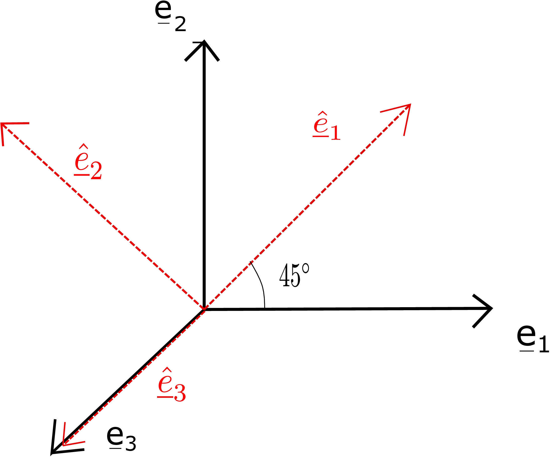
will be the traction on a plane with normal \(\ve {n}=\hat {\ve
{e}}_1\) where \( \brc {\hat {\ve {e}}_{1}, \hat {\ve {e}}_{2}, \hat
{\ve {e}}_{3}}\) is obtained from rotation of \(\brc {\ve {e}_{1}, \ve
{e}_{2}, \ve {e}_{3}}\) about \( \ve {e}_3\) by \( 45^\circ \)
(see the figure below)? What are the normal and shear components of
traction on this plane?
Solution: We simply have to use the formula
\(\ve {t}^n=\msum {i}\ve {t}^{i}\brc {\ve {n}\cdot \ve {e}_i}\).
Keep in mind that the above is a tensor formula. To use it, we must write every quantity involved in the above formula in the same coordinate system! Let us use \(\brc {\ve {e}_{1}, \ve {e}_{2}, \ve {e}_{3}}\) coordinate system here:
\(\Rightarrow \sbk {\ve {n}}_{\brc {\ve {e}_{1}, \ve {e}_{2}, \ve {e}_{3}}} = \sbk {\hat {\ve {e}}_1}_{\brc {\ve {e}_{1}, \ve {e}_{2}, \ve {e}_{3}}} = \begin {bmatrix} 1/\sqrt {2}\\1/\sqrt {2}\\0 \end {bmatrix}\).
Therefore \begin {align*} \begin {split} \sbk {\ve {t}^n} = \msum {i}\sbk {\ve {t}^i} \brc {\sbk {\ve {n}}\cdot \sbk {\ve {e}_i}}= 1/\sqrt {2} \begin {bmatrix} 0\\1\\0 \end {bmatrix}+ 1/\sqrt {2} \begin {bmatrix} 1\\5\\7 \end {bmatrix}+ 0\begin {bmatrix} 0\\7\\9 \end {bmatrix}= 1/\sqrt {2}\begin {bmatrix} 1\\6\\7 \end {bmatrix}. \end {split} \end {align*}
CAUTION: If you use \( \sbk {\ve {n}}=\begin {bmatrix} 1\\0\\0 \end {bmatrix}\), you will get wrong result! Never mix the coordinate system! Either use \(\brc {\ve {e}_{1}, \ve {e}_{2}, \ve {e}_{3}}\) for all or use \( \brc {\hat {\ve {e}}_{1}, \hat {\ve {e}}_{2}, \hat {\ve {e}}_{3}}\) for all. The final result for \(\ve {t}^n\) will be in the coordinate system that you choose. In order to get the normal component of traction, we need to find \(\underline {t}^n\cdot \underline {n}\) or \(\underline {t}^{\hat {1}}\cdot \underline {\hat {e}}_1\) which when expressed in \(\brc {\ve {e}_{1}, \ve {e}_{2}, \ve {e}_{3}}\) coordinate system yields \begin {equation} 1/\sqrt {2}\begin {bmatrix} 1\\6\\7 \end {bmatrix}\cdot \begin {bmatrix} 1/\sqrt {2}\\1/\sqrt {2}\\0 \end {bmatrix}=\frac {7}{2}.\nonumber \end {equation} One can likewise obtain the shear components by taking the dot product of traction vector with \(\underline {\hat {e}}_2\) and \(\hat {\underline {e}}_3\).
Q3. Show that the component of a traction vector on \(\ve {n}\)-plane in the direction \(\ve {m}\) equals the component of the traction on \(\ve {m}\)-plane in the direction \(\ve {n}\), i.e, \(\underline {t}^n\cdot \underline {m} = \underline {t}^m\cdot \underline {n}\).
Solution: To prove this, we will use the definition of stress tensor as follows: \begin {align*} \begin {split} \ve {t}^n\cdot \ve {m} &= \brc {\matr {\sigma }\;\ve {n}}\cdot \ve {m} \\ &= \ve {n}\cdot \brc {\matr {{\sigma }}^T\;\ve {m}} \\ &=\ve {n}\cdot \brc {\matr {{\sigma }}\;\ve {m}} \text { (due to symmetry of $\matr {\sigma }$ which will be proved later)}\\ &=\ve {n}\cdot \ve {t}^m \; . \end {split} \end {align*}
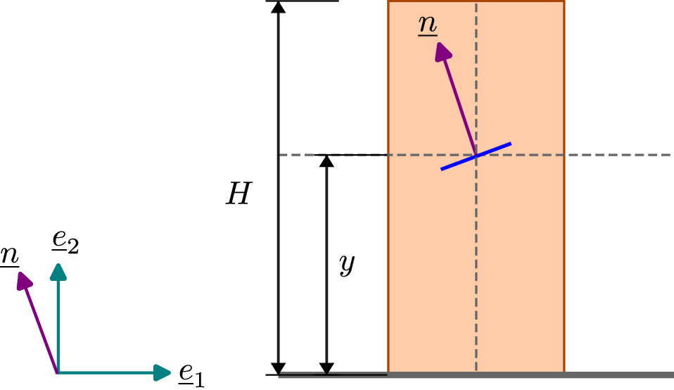
Q4. Consider a vertical bar having mass density \(\rho \). Assume its length be to \(H\) and is subjected to uniform body force due to gravity. Find the traction vector on an infinitesimal internal section of the bar located at the center of its cross-section with outward normal \[ \ve {n} = -\sin \theta \; \ve {e}_1 + \cos \theta \; \ve {e}_2\] and at a height of \(y\) from the base (see figure). Also find the normal and tangential components of the traction vector on this plane.
Solution:
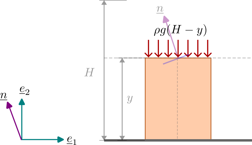
Taking a horizontal section at height \(y\) and writing force balance of top part of bar yields \[ \sbk {\ve {t}^2} = \begin {bmatrix} 0 \\ -\rho g (H-y)\\0 \end {bmatrix}. \] Similarly taking a vertical section all along the bar and doing force balance either of left or right portion of the bar yields \[\sbk {\ve {t}^1} = \begin {bmatrix} 0 \\ 0\\0 \end {bmatrix}. \] One can likewise show that \(\sbk {\ve {t}^3}\) also vanishes although it turns out this information is not required. In order to obtain traction on an infinitesimal inclined plane at the center of the horizontal section of the bar, we can use the tetrahedron formula, i.e., \begin {align*} \sbk {\ve {t}^n} &= \msum {i}\sbk {\ve {t}^i} \brc {\sbk {\ve {n}}\cdot \sbk {\ve {e}_i}}\\ &= \begin {bmatrix} 0\\0\\0 \end {bmatrix} (-\sin \theta ) + \begin {bmatrix} 0\\ -\rho g (H-y) \\0\end {bmatrix} (\cos \theta ) + \begin {bmatrix} \underline {t}^3\end {bmatrix}~0 = \begin {bmatrix} 0\\ -\rho g (H-y) \cos \theta \\0\end {bmatrix}. \end {align*}
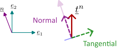
The normal component of traction vector is given by the projection of \(\ve {t}^n\) along \(\ve {n}\): \begin {align*} t_\text {normal} &= \ve {t}^n \cdot \ve {n} \\ &= - \rho g (H-y) \cos \theta \; \brc {\ve {e}_2 \cdot \ve {n}} = - \rho g (H-y) \cos ^2 \theta . \end {align*}
The shear or tangential component of traction can then be obtained as follows: \begin {align*} t_{\text {tangential}} &= \ve {t}^{n} \cdot \ve {n}^{\perp } \\ &= - \rho g (H-y) \cos \theta \; \ve {e}_2 \cdot \brc {\cos \theta \; \ve {e}_1 + \sin \theta \; \ve {e}_2} = - \rho g (H-y) \cos \theta \sin \theta \end {align*}
where \(\ve {n}^{\perp }\) is a unit vector perpendicular to \(\ve {n}\) and lies in the plane of inclined section.
Q5. Suppose the stress matrix in (\(\underline {e}_1\), \(\underline {e}_2\), \(\underline {e}_3\)) coordinate system is given by \begin {equation} \begin {bmatrix} \underline {\underline {\sigma }} \end {bmatrix}_{(\underline {e}_1, \underline {e}_2, \underline {e}_3)}= \begin {bmatrix} \frac {1}{\sqrt {2}} & \frac {1}{\sqrt {2}} & 0\\ \frac {1}{\sqrt {2}} & \frac {1}{\sqrt {2}} & 0\\ 0 & 0 & 1 \end {bmatrix}.\nonumber \end {equation} Think of a new coordinate system which is obtained by rotation of (\(\underline {e}_1\), \(\underline {e}_2\), \(\underline {e}_3\)) coordinate system by \(45\degree \) about \(\underline {e}_3\) as in problem 2 above. Find the stress matrix in the new coordinate system.
First, we need to find the rotation matrix. As derived earlier, this rotation matrix will be \begin {equation} \begin {bmatrix} \underline {\underline {R}} \end {bmatrix}_{(\underline {e}_1, \underline {e}_2, \underline {e}_3)}= \begin {bmatrix} cos(45\degree ) & -sin(45\degree ) & 0\\ sin(45\degree ) & cos(45\degree ) & 0\\ 0 & 0 & 1 \end {bmatrix}= \begin {bmatrix} \frac {1}{\sqrt {2}} & -\frac {1}{\sqrt {2}} & 0\\ \frac {1}{\sqrt {2}} & \frac {1}{\sqrt {2}} & 0\\ 0 & 0 & 1 \end {bmatrix}.\nonumber \end {equation} Now, we can apply the formula for stress matrix transformation, i.e., equation \eqref{2_stress_transformation}. We get \begin {equation} \begin {bmatrix} \underline {\underline {\sigma }} \end {bmatrix}_{(\underline {\hat e}_1, \underline {\hat e}_2, \underline {\hat e}_3)}= \begin {bmatrix} \sqrt {2} & 0& 0\\ 0 & 0 & 0\\ 0 & 0 & 1 \end {bmatrix}.\nonumber \end {equation} From this, we observe that the second column has all zeros which implies that there is no traction on \(\underline {\hat e}_2\) plane. The traction on \(\underline {\hat e}_1\) plane has just the first component non-zero - only normal component of traction acts here. Let us verify the new stress matrix by directly finding the traction on one of the planes say \(\underline {\hat e}_2\) plane: \begin {equation} \underline {t}^{\hat 2}= \sum _{i=1}^3 \underline {t}^i~(\underline {\hat e}_2\cdot \underline {e}_i).\nonumber \end {equation} This is a vector equation. Let’s write this down in (\(\underline {e}_1, \underline {e}_2, \underline {e}_3\)) coordinate system. To know the traction columns, we look at the stress matrix given in (\(\underline {e}_1, \underline {e}_2, \underline {e}_3\)) coordinate system. To obtain the column form of \(\underline {\hat e}_2\), we look at the second column of our rotation matrix. Thus
This zero column represents \(\underline {t}^{\hat 2}\) in (\(\underline {e}_1, \underline {e}_2, \underline {e}_3\)) coordinate system. But being a ‘zero column’ means that its representation in any coordinate system will also be a zero column. Therefore, the \(2^{nd}\) column of \(\begin {bmatrix} \underline {\underline {\sigma }} \end {bmatrix}_{(\underline {\hat e}_1, \underline {\hat e}_2, \underline {\hat e}_3)}\) turned out to be a zero column earlier.
Q6. A tapered beam is clamped at one end and subjected to a transverse load (along \(\ve {e}_2\)) at the other end. Think of a point A on the top slanted surface of the beam. What can you say about the state of stress at point A? Suppose we know \(\hat {\sigma }_{11}\) at point A. Can we find the components \(\tau _{21},\sigma _{11},\hat {\tau }_{21}\) at point A? Assume that the internal traction on any plane and at any point in the body has no component along \(\ve {e}_3\). [AMS, LSS]
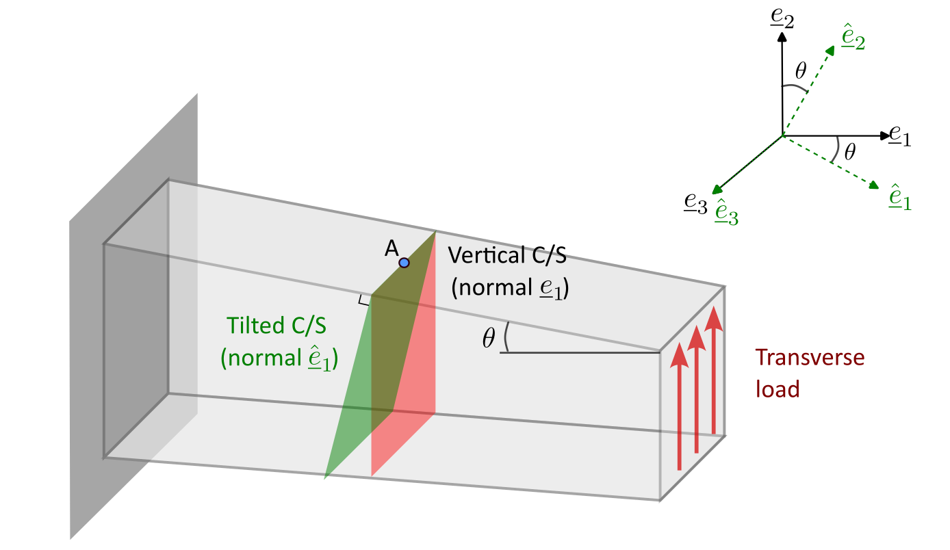
Solution: Notice that point A lies on the slanted surface where no external load is being applied! Furthermore, the slanted surface has normal \(\hat {\ve {e}}_2\).
This implies \( \ve {t}^{\hat {2}}=\ve {0}\) at point A (this does not mean \( \ve {t}^2=\ve {0}.\))
If we write the stress matrix in a coordinate system of (\( \hat {\ve {e}}_{1}, \hat {\ve {e}}_{2}, \hat {\ve {e}}_{3}\)), then the \(2^{nd}\) column will be zero (\(\ve {t}^{\hat {2}}=\ve {0}\)). Furthermore, the third row will also be zero since tractions have zero components along \(\ve {e}_3\) (which equals \(\hat {\ve {e}}_3\)). Thus \begin {align*} \sbk {\matr {\sigma }\brc {A}}_{\brc {\hat {\ve {e}}_{1}, \hat {\ve {e}}_{2},\hat {\ve {e}}_{3}}} = \begin {bmatrix} X & 0 & X \\ X & 0& X \\0 & 0 & 0 \end {bmatrix}. \end {align*}
We will see in next chapter that the stress matrix is also symmetric. Hence
\(\sbk {\matr {\sigma } (A)}_{\brc {\hat {\ve {e}}_{1}, \hat {\ve {e}}_{2},\hat {\ve {e}}_{3}}}= \begin {bmatrix} X & 0 & 0 \\ 0 & 0& 0 \\0 & 0 & 0 \end {bmatrix}\).
Hence, \(\hat {\sigma }_{11}\) is the only non-zero quantity! Note that \(\hat {\tau }_{21}\)=0 (since \(\hat {\tau }_{12}=0)\). From here, we can then transform the stress matrix to \(\brc {\ve {e}_{1}, \ve {e}_{2}, \ve {e}_{3}}\) coordinate system.
If \(\hat {\ve {e}}_i=\matr {R}\;\ve {e}_i \;\Rightarrow \sbk {\matr {R}}_{\brc {\ve {e}_{1}, \ve {e}_{2}, \ve {e}_{3}}}=\begin {bmatrix} \cos \theta & \sin \theta & 0 \\ -\sin \theta & \cos \theta & 0 \\ 0 & 0 & 1 \end {bmatrix}\)
\( \text {and}~ \hat {\sbk {\matr {\sigma }}} = \sbk {\matr {R}}^T\sbk {\matr {\sigma }}\sbk {\matr {R}}\)
\begin {align*} \Rightarrow \sbk {\matr {\sigma }} & = \sbk {\matr {R}} \hat {\sbk {\matr {\sigma }}}\sbk {\matr {R}}^T\\ & = \begin {bmatrix} c\theta & s\theta & 0 \\ -s\theta & c\theta & 0 \\ 0 & 0& 1 \end {bmatrix}\begin {bmatrix} \hat {\sigma }_{11} & 0 & 0\\ 0 & 0& 0\\ 0 & 0 & 0 \end {bmatrix} \begin {bmatrix} c\theta & - s\theta & 0\\ s\theta & c\theta & 0\\ 0 & 0& 1 \end {bmatrix} = \begin {bmatrix} \hat {\sigma }_{11}\cos ^2\theta & -\hat {\sigma }_{11}s\theta c\theta &0\\ -\hat {\sigma }_{11}s\theta c\theta & \hat {\sigma }_{11} \sin ^2\theta & 0\\ 0 & 0 & 0 \end {bmatrix}\\ \Rightarrow \sigma _{11} &= \hat {\sigma }_{11}\cos ^2 \theta ,~ \tau _{12} =\tau _{21}=-\hat {\sigma }_{11}\sin \theta \cos \theta ,~ \sigma _{22} = \hat {\sigma }_{11}\sin ^2 \theta . \end {align*}
There is another way to obtain these components. Let us first obtain the traction on \(\ve {e}_1\)-plane using \(\ve {t}^{1} = \matr {\sigma }\;\ve {e}_1\). As we have \(\sbk {\matr {\sigma }}\) readily available in the ‘hat’ coordinate system, we can write the tensor formula to obtain \(\sbk {\ve {t}^1}\) in the ‘hat’-coordinate system.
\(\Rightarrow \sbk {\ve
{t}^{1}}_{\brc {\hat {\ve {e}}_{1}, \hat {\ve {e}}_{2}, \hat {\ve
{e}}_{3}}} = \sbk {\matr {\sigma }}_{\brc {\hat {\ve {e}}_{1}, \hat
{\ve {e}}_{2}, \hat {\ve {e}}_{3}}} \sbk {\ve {e}_1}_{\brc {\hat {\ve
{e}}_{1}, \hat {\ve {e}}_{2}, \hat {\ve {e}}_{3}}} = \begin {bmatrix}
\hat {\sigma }_{11} & 0 & 0\\ 0 & 0 & \\ 0 & 0
& 0 \end {bmatrix}\begin {bmatrix} \cos \theta \\ \sin \theta \\ 0
\end {bmatrix}=\begin {bmatrix} \hat {\sigma }_{11}\cos \theta \\0\\0
\end {bmatrix}\)
\(\Rightarrow \sigma _{11}=\ve {t}^{1}\cdot \ve {e}_1 = \sbk {\ve
{t}^{1}}_{\brc {\hat {\ve {e}}_{1}, \hat {\ve {e}}_{2}, \hat {\ve
{e}}_{3}}}\cdot \sbk {\ve {e}_1}_{\brc {\hat {\ve {e}}_{1}, \hat {\ve
{e}}_{2}, \hat {\ve {e}}_{3}}} =\begin {bmatrix} \hat {\sigma
}_{11}\cos \theta \\ 0\\ 0 \end {bmatrix}\cdot \begin {bmatrix} \cos
\theta \\ \sin \theta \\ 0 \end {bmatrix}=\hat {\sigma }_{11} \cos
^2\theta \)!
\(\textbf {Caution}\): Don’t make a mistake by writing \(\sbk {\ve {e}_1}_{\brc {\hat {\ve {e}}_{1}, \hat {\ve {e}}_{2}, \hat {\ve {e}}_{3}}}=\begin {bmatrix} 1 \\ 0 \\ 0 \end {bmatrix}\).
Q7.
The state of stress at a point is given by \(\sbk {\matr {\sigma }} =
\begin {bmatrix} \sigma _{11} &2& 1\\ 2 & 0 & 3\\ 1
& 3 & 0 \end {bmatrix}\).
What should be \(\sigma _{11}\) such that there is at least one plane at that point on which the traction vanishes?
Also, find the corresponding plane normal.
Solution: We basically want \(\matr {\sigma }\;\ve {n} = \ve {0}\) for at least one \(\ve {n}\)!
or \(\begin {bmatrix} \sigma _{11} &2& 1\\2 & 0 & 3\\1 & 3 & 0 \end {bmatrix}\begin {bmatrix}n_1 \\ n_2 \\ n_3 \end {bmatrix} = \begin {bmatrix}0\\0\\0 \end {bmatrix} \)
From matrix property, we know that this happens only when the determinant of the matrix vanishes \begin {align*} \Rightarrow \det \brc {\sbk {\matr {\sigma }}} = \sigma _{11}\times \sbk {-9}-2\times \sbk {-3}+1\times 6 &=0\\ \Rightarrow -9\sigma _{11}+6 +6 &=0 ~\text {or}~ \sigma _{11} = 4/3. \end {align*}
The plane normal \(\ve {n}\) would simply be the eigenvector of above matrix corresponding to zero eigenvalue.
Q8. Suppose a body is under stress and the stress tensor at an arbitrary point \(\underline x\) in the body is denoted by \(\underline {\underline {\sigma }}\). Further, suppose the stressed body is then rigidly rotated where the corresponding rotation is denoted by the tensor \(\underline {\underline {R}}\). Let us think of a coordinate system attached with the stressed body which also rotates when the stressed body rotates.
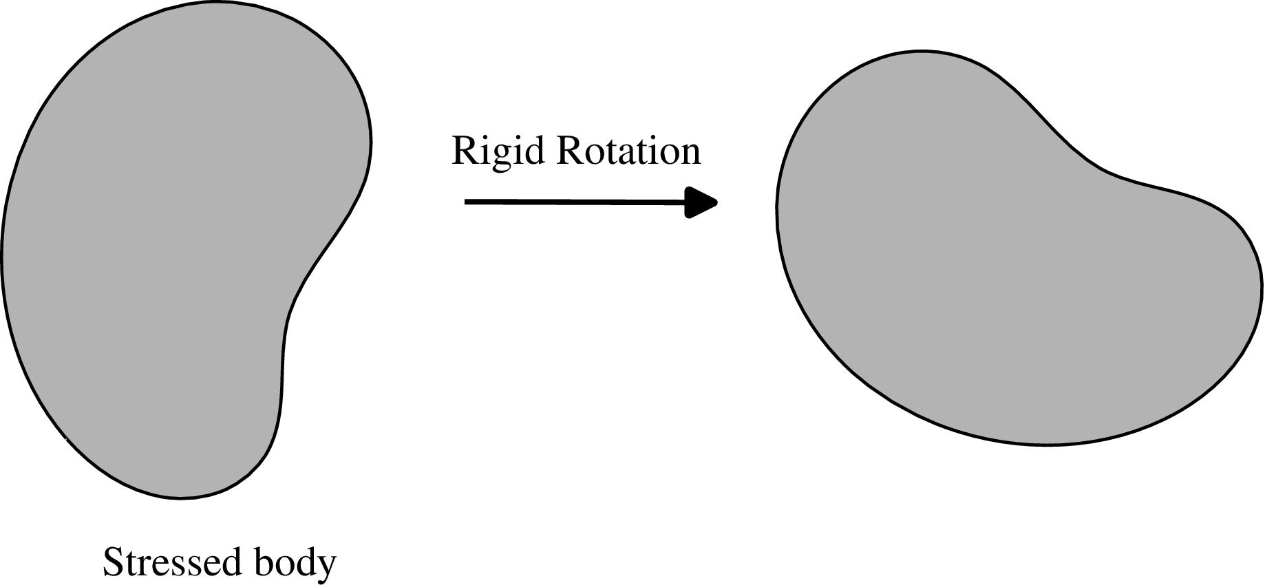
(i) What can you say about the stress matrix in the body before and after rotation in the coordinate system
attached with the body?
(ii) What happens to the stress matrix in a fixed coordinate system not attached to the body?
(iii) What happens to the stress tensor due to rotation of the stressed body?
Solution: (i)
Keep in mind that rigid rotation does not induce extra stain in the body! Further, stress being proportional to
strain, stress components in a body-fixed coordinate system should not change! Hence, there will be no change in the
stress matrix in a coordinate system fixed to the body!
(ii)
Suppose the rotation tensor for rigid rotation is \(\matr {R}\).
Furthermore, let \(\matr {\sigma }\;=\;\msum {i} \ve {t}^i \otimes
\;\ve {e}_i\) before rotation! Concentrate on these three
planes with their normals along coordinate axis. After rotation \begin
{align*} \ve {e}_i \;\rightarrow \;\matr {R}\;\ve {e}_i,\quad \ve {t}^i
\;\rightarrow \;\matr {R}\;\ve {t}^i. \end {align*}
So, \begin {align*} \matr {\sigma }^R \text {(after rotation)}\;&=\;\msum {i} \ve {t}^{i,R} \otimes \ve {e}^R_{i} =\;\msum {i}\;\matr {R}\;\ve {t}^i \otimes \matr {R}\;\ve {e}_i =\;\matr {R}\brc {\msum {i}\ve {t}^i \otimes \ve {e}_i} \matr {R}^T=\matr {R}\;\matr {\sigma }\;\matr {R}^T. \end {align*}
(iii) It transforms to \(\matr {R}\;\matr {\sigma }\;\matr {R}^T\). In a fixed coordinate system (say \(\ve {E}_1-\ve {E}_2-\ve {E}_3\)): \begin {align*} \sbk {\matr {\sigma }^R}_{[\ve {E}_1-\ve {E}_2-\ve {E}_3]}\;&=\;\sbk {\matr {R}\;\matr {\sigma }\;\matr {R}^T}_{[\ve {E}_1-\ve {E}_2-\ve {E}_3]}\\ &=\;\sbk {\matr {R}}_{[\ve {E}_1-\ve {E}_2-\ve {E}_3]}\sbk {\matr {\sigma }}_{[\ve {E}_1-\ve {E}_2-\ve {E}_3]}\sbk {\matr {R}^T}_{[\ve {E}_1-\ve {E}_2-\ve {E}_3] }. \end {align*}
Hence, the stress matrix in (\(\ve {E}_1-\ve {E}_2-\ve {E}_3\)) coordinate system changes!
\([\underline {\underline {\sigma }}]_{(e_1,e_2,e_3)}\) = \(\begin {bmatrix}\sqrt {2}&0&0\\1&0&0\\0&1&0\end {bmatrix}\)
\([\underline {\underline {\sigma }}]_{(\hat {\underline e}_1,\hat {\underline e}_2,\hat {\underline e}_3)}\) = \(\underbrace {[\underline {\underline {R}}][\underline {\underline {\sigma }}][\underline {\underline {R}}]^T}_{(\underline e_1,\underline e_2,\underline e_3)}\)
Which of the following is true about \(\underline {\underline {R}}\) in the above equation?
\([\underline {\underline {\sigma }}]_{(e_1,e_2,e_3)}\) = \(\begin {bmatrix}10&50 &- 50\\50&0&0\\ - 50&0&0\end {bmatrix}\).
What will be the value of normal component of traction on a plane whose normal is \(\underline {e}_1'\) (it is in the direction of \(\underline {e}_1+2\underline {e}_2+3\underline {e}_3\))?
\(\underline t^a = -1\underline e_1 + \sqrt {3}\underline e_2\), \(\underline t^b = \sqrt {3}\underline e_1 + 1\underline e_2\), \(\underline t^c = 10\underline e_3\).
Here \(a =\frac {1}{2} (\sqrt {3}\underline e_1 + \underline e_2)\), \(b = \frac {1}{2}(-\underline e_1 + \sqrt {3}\underline e_2)\), \(c = \underline e_3\) and (\(\underline e_1\), \(\underline e_2\), \(\underline e_3\)) are the standard basis vectors of a Cartesian coordinate system.
∗For simplicity, we have assumed here that we have the same traction at every point on this section although that is not the usual case.
†Note that we always consider outward normals.
‡In most books, \(\tau _{ij}\) denotes the \(j^{th}\) component of traction on \(i^{th}\) plane but we will follow our convention since it comes out this way naturally. Our convention also aligns with the convention for components of other stress measures such as the first Piola-Kirchhoff stress tensor in nonlinear elasticity.