5 Introduction to Quantum Mechanics
5.1 The Schrödinger Equation
Consider a particle of mass \(m\), constrained to move along the \(x\)-axis, subject to some specified force \(F(x,t)\). Classical mechanics seeks to determine the position \(x(t)\) at any time — from which velocity \(v = dx/dt\), momentum \(p = mv\), and kinetic energy \(T = \tfrac{1}{2}mv^2\) all follow. For conservative systems the force derives from a potential energy function:
\[ F = -\frac{\partial V}{\partial x}, \tag{5.1}\]
and Newton’s second law \(m\,d^2x/dt^2 = -\partial V/\partial x\), together with initial conditions, determines \(x(t)\).
Quantum mechanics approaches this problem differently. The goal is the particle’s wave function \(\Psi(x,t)\), obtained by solving the Schrödinger equation:
\[ \boxed{i\hbar\frac{\partial\Psi}{\partial t} = -\frac{\hbar^2}{2m}\frac{\partial^2\Psi}{\partial x^2} + V\Psi} \tag{5.2}\]
where \(i = \sqrt{-1}\) and \(\hbar\) is the reduced Planck constant:
\[ \hbar = \frac{h}{2\pi} = 1.054572\times10^{-34}\ \text{J s}. \tag{5.3}\]
5.2 The Statistical Interpretation
But what exactly is this “wave function,” and what does it do for you once you’ve got it? After all, a particle, by its nature, is localized at a point, whereas the wave function (as its name suggests) is spread out in space (it’s a function of \(x\), for any given time \(t\)). How can such an object represent the state of a particle? The answer is provided by Born’s statistical interpretation of the wave function, which says that \(|\Psi(x,t)|^2\) gives the probability density for finding the particle at point \(x\), at time \(t\) - or, more precisely,
\[ \int_a^b |\Psi(x,t)|^2\,dx \tag{5.4}\]
is the probability of finding the particle between \(a\) and \(b\), at time \(t\).
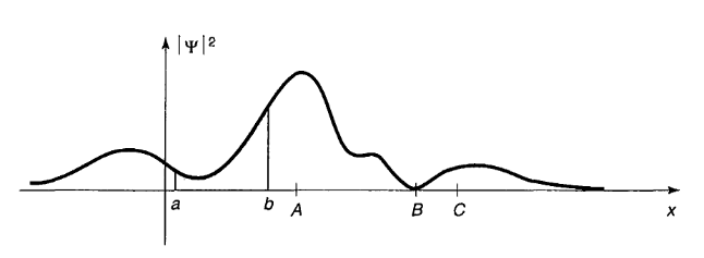
Probability is the area under the graph of \(|\Psi|^2\). For the wave function in Fig. 5.1, you would be quite likely to find the particle in the vicinity of point \(A\), where \(|\Psi|^2\) is large, and relatively unlikely to find it near point \(B\).
The statistical interpretation introduces a kind of indeterminacy into quantum mechanics, for even if you know everything the theory has to tell you about the particle (to wit: its wave function), still you cannot predict with certainty the outcome of a simple experiment to measure its position - all quantum mechanics has to offer is statistical information about the possible results. This indeterminacy has been profoundly disturbing to physicists and philosophers alike, and it is natural to wonder whether it is a fact of nature, or a defect in the theory.
Suppose I do measure the position of a particle, and I find it to be at point \(C\). Question: Where was the particle just before I made the measurement? There are three plausible answers to this question, and they serve to characterize the main schools of thought regarding quantum indeterminacy:
The realist position: The particle was at \(C\). This certainly seems like a sensible response, and it is the one Einstein advocated. Note, however, that if this is true then quantum mechanics is an incomplete theory, since the particle really was at \(C\), and yet quantum mechanics was unable to tell us so. To the realist, indeterminacy is not a fact of nature, but a reflection of our ignorance. Evidently some additional information, known as a hidden variable, is needed to provide a complete description of the particle.
The orthodox position: The particle wasn’t really anywhere. It was the act of measurement that forced the particle to take a stand. This view, the so-called Copenhagen interpretation, is associated with Bohr and his followers. Among physicists it has always been the most widely accepted position. Note, however, that if it is correct there is something very peculiar about the act of measurement - something that over half a century of debate has done precious little to illuminate.
The agnostic position: Refuse to answer. This is not quite as silly as it sounds - after all, what sense can there be in making assertions about the status of a particle before a measurement, when the only way of knowing whether you were right is precisely to conduct a measurement, in which case what you get is no longer “before the measurement?” It is metaphysics to worry about something that cannot, by its nature, be tested. For decades this was the fall-back position of most physicists.
Until fairly recently, all three positions had their partisans. But in 1964 John Bell astonished the physics community by showing that it makes an observable difference whether the particle had a precise, though unknown, position prior to the measurement, or not. Bell’s discovery effectively eliminated agnosticism as a viable option, and made it an experimental question whether the realist or orthodox choice is correct. I’ll return to this story at the end of the book, when you will be in a better position to appreciate Bell’s argument; for now, suffice it to say that the experiments have decisively confirmed the orthodox interpretation: A particle simply does not have a precise position prior to measurement, any more than the ripples on a pond do; it is the measurement process that insists on one particular number, and thereby in a sense creates the specific result, limited only by the statistical weighting imposed by the wave function.
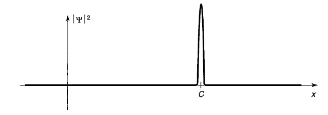
What if I made a second measurement, immediately after the first? Would I get \(C\) again, or does the act of measurement cough up some completely new number each time? On this question everyone is in agreement: A repeated measurement on the same particle must return the same value. Indeed, it would be tough to prove that the particle was really found at \(C\) in the first instance, if this could not be confirmed by immediate repetition of the measurement. How does the orthodox interpretation account for the fact that the second measurement is bound to yield the value \(C\)? Evidently the first measurement radically alters the wave function, so that it is now sharply peaked about \(C\) (Fig. 5.2). We say that the wave function collapses, upon measurement, to a spike at the point \(C\); it soon spreads out again, in accordance with the Schrödinger equation, so the second measurement must be made quickly. There are, then, two entirely distinct kinds of physical processes: “ordinary” ones, in which the wave function evolves in a leisurely fashion under the Schrödinger equation, and “measurements,” in which it suddenly and discontinuously collapses.
5.3 Normalization
We return now to the statistical interpretation of the wave function (Equation Eq. 5.4), which says that \(|\Psi(x,t)|^2\) is the probability density for finding the particle at point \(x\), at time \(t\). It follows that the integral of \(|\Psi|^2\) must be 1 (the particle’s got to be somewhere):
\[ \int_{-\infty}^{\infty} |\Psi(x,t)|^2\,dx = 1 \tag{5.5}\]
Without this, the statistical interpretation would be nonsense.
However, this requirement should disturb you: After all, the wave function is supposed to be determined by the Schrödinger equation - we can’t go imposing an extraneous condition on \(\Psi\) without checking that the two are consistent. Well, a glance at Equation Eq. 5.2 reveals that if \(\Psi(x,t)\) is a solution, so too is \(A\Psi(x,t)\), where \(A\) is any complex constant. What we must do, then, is pick this undetermined multiplicative factor so as to ensure that Equation Eq. 5.5 is satisfied. This process is called normalizing the wave function. For some solutions to the Schrödinger equation the integral is infinite; in that case no multiplicative factor is going to make it 1. The same goes for the trivial solution \(\Psi = 0\). Such non-normalizable solutions cannot represent particles, and must be rejected. Physically realizable states correspond to the square-integrable solutions to Schrödinger’s equation.
But wait a minute! Suppose I have normalized the wave function at time \(t = 0\). How do I know that it will stay normalized, as time goes on, and \(\Psi\) evolves? You can’t keep renormalizing the wave function, for then \(A\) becomes a function of \(t\), and you no longer have a solution to the Schrödinger equation. Fortunately, the Schrödinger equation has the remarkable property that it automatically preserves the normalization of the wave function - without this crucial feature the Schrödinger equation would be incompatible with the statistical interpretation, and the whole theory would crumble.
This is important, so we’d better pause for a careful proof. To begin with,
\[ \frac{d}{dt}\int_{-\infty}^{\infty} |\Psi(x,t)|^2\,dx = \int_{-\infty}^{\infty}\frac{\partial}{\partial t}\bigl(\Psi^*\Psi\bigr)\,dx \tag{5.6}\]
(Note that the integral is a function only of \(t\), so I use a total derivative in the first expression, but the integrand is a function of \(x\) as well as \(t\), so it’s a partial derivative in the second one.) By the product rule,
\[ \frac{\partial}{\partial t}|\Psi|^2 = \Psi^*\frac{\partial \Psi}{\partial t} +\Psi\frac{\partial \Psi^*}{\partial t} \tag{5.7}\]
Now the Schrödinger equation says that
\[ \frac{\partial \Psi}{\partial t} = \frac{i\hbar}{2m}\frac{\partial^2\Psi}{\partial x^2} -\frac{i}{\hbar}V\Psi \tag{5.8}\]
and hence also, taking the complex conjugate,
\[ \frac{\partial \Psi^*}{\partial t} = -\frac{i\hbar}{2m}\frac{\partial^2\Psi^*}{\partial x^2} +\frac{i}{\hbar}V\Psi^* \tag{5.9}\]
So
\[ \frac{\partial}{\partial t}|\Psi|^2 = \frac{i\hbar}{2m} \left( \Psi^*\frac{\partial^2\Psi}{\partial x^2} -\Psi\frac{\partial^2\Psi^*}{\partial x^2} \right) \tag{5.10}\]
The integral in Equation Eq. 5.6 can now be evaluated explicitly:
\[ \frac{d}{dt}\int_{-\infty}^{\infty} |\Psi(x,t)|^2\,dx = \frac{i\hbar}{2m}\left[\Psi^*\frac{\partial \Psi}{\partial x} -\Psi\frac{\partial \Psi^*}{\partial x}\right]_{-\infty}^{\infty} \tag{5.11}\]
But \(\Psi(x,t)\) must go to zero as \(x\) goes to \(\pm\infty\) - otherwise the wave function would not be normalizable. It follows that
\[ \frac{d}{dt}\int_{-\infty}^{\infty} |\Psi(x,t)|^2\,dx = 0 \tag{5.12}\]
and hence that the integral is constant, independent of time; if \(\Psi\) is normalized at \(t=0\), it stays normalized for all future time. QED.
At time \(t=0\) a particle is represented by the wave function
\[ \Psi(x,0)= \begin{cases} Ax/a, & 0 < x < a, \\ A(b-x)/(b-a), & a < x < b, \\ 0, & \text{otherwise}, \end{cases} \]
where \(A\), \(a\), and \(b\) are constants.
Normalize (that is, find \(A\), in terms of \(a\) and \(b\)).
Sketch \(\Psi(x,0)\), as a function of \(x\).
Where is the particle most likely to be found, at \(t=0\)?
What is the probability of finding the particle to the left of \(a\)? Check your result in the limiting cases \(b=a\) and \(b=2a\).
What is the expectation value of \(x\)?
Consider the wave function
\[ \Psi(x,t)=A e^{-a x^2}e^{-i\omega t} \]
where \(A\), \(a\), and \(\omega\) are positive real constants. (We’ll see in Chapter 2 what potential \(V\) actually produces such a wave function.)
Normalize \(\Psi\).
Determine the expectation values of \(x\) and \(x^2\).
Find the standard deviation of \(x\). Sketch the graph of \(|\Psi|^2\), as a function of \(x\), and mark the points \(\langle x \rangle+\sigma\) and \(\langle x \rangle-\sigma\), to illustrate the sense in which \(\sigma\) represents the spread in \(x\). What is the probability that the particle would be found outside this range?
5.4 Momentum
For a particle in state \(\Psi\), the expectation value of x is
\[ \langle x \rangle = \int_{-\infty}^{\infty} x |\Psi(x,t)|^2\,dx \tag{5.13}\]
What exactly does this mean? It emphatically does not mean that if you measure the position of one particle over and over again, the integral is the average of the results you’ll get. On the contrary: The first measurement (whose outcome is indeterminate) will collapse the wave function to a spike at the value actually obtained, and the subsequent measurements (if they’re performed quickly) will simply repeat that same result. Rather, \(\langle x \rangle\) is the average of measurements performed on particles all in the state \(\Psi\), which means that either you must find some way of returning the particle to its original state after each measurement, or else you have to prepare a whole ensemble of particles, each in the same state \(\Psi\), and measure the positions of all of them: \(\langle x \rangle\) is the average of these results. In short, the expectation value is the average of repeated measurements on an ensemble of identically prepared systems, not the average of repeated measurements on one and the same system.
Now, as time goes on, \(\langle x \rangle\) will change, and we might be interested in knowing how fast it moves. Referring to Equations Eq. 5.10 and Eq. 5.13, we see that
\[ \frac{d\langle x \rangle}{dt} = \frac{i\hbar}{2m}\int_{-\infty}^{\infty} \left( x\Psi\frac{\partial^2\Psi^*}{\partial x^2} -x\Psi^*\frac{\partial^2\Psi}{\partial x^2} \right)dx \tag{5.14}\]
This expression can be simplified using integration by parts:
\[ \frac{d\langle x \rangle}{dt} = \frac{i\hbar}{2m}\int_{-\infty}^{\infty} \left( \Psi\frac{\partial\Psi^*}{\partial x} -\Psi^*\frac{\partial\Psi}{\partial x} \right)dx \tag{5.15}\]
(I used the fact that \(dx/dx = 1\), and threw away the boundary term, on the ground that \(\Psi\) goes to zero at infinity.) Performing another integration by parts, on the second term, we conclude:
\[ \frac{d\langle x \rangle}{dt} = \frac{\hbar}{m}\,\mathrm{Im}\!\int_{-\infty}^{\infty}\Psi^*\frac{\partial\Psi}{\partial x}\,dx \tag{5.16}\]
What are we to make of this result? Note that we’re talking about the velocity of the expectation value of \(x\), which is not the same thing as the velocity of the particle. Nothing we have seen so far would enable us to calculate the velocity of a particle. It is not even clear what velocity means in quantum mechanics: If the particle doesn’t have a determinate position prior to measurement, neither does it have a well-defined velocity. All we could reasonably ask for is the probability of getting a particular value. We’ll see in Chapter 3 how to construct the probability density for velocity, given \(\Psi\); for our present purposes it will suffice to postulate that the expectation value of the velocity is equal to the time derivative of the expectation value of position:
\[ \langle v \rangle = \frac{d\langle x \rangle}{dt} \tag{5.17}\]
Equation Eq. 5.16 tells us, then, how to calculate \(\langle v \rangle\) directly from \(\Psi\).
Actually, it is customary to work with momentum (\(p = mv\)), rather than velocity:
\[ \langle p \rangle = m\langle v \rangle = -i\hbar \int_{-\infty}^{\infty}\Psi^*\frac{\partial\Psi}{\partial x}\,dx \tag{5.18}\]
Let me write the expressions for \(\langle x \rangle\) and \(\langle p \rangle\) in a more suggestive way:
\[ \langle x \rangle = \int_{-\infty}^{\infty}\Psi^* x \Psi\,dx \tag{5.19}\]
\[ \langle p \rangle = \int_{-\infty}^{\infty}\Psi^*\left(-i\hbar\frac{\partial}{\partial x}\right)\Psi\,dx \tag{5.20}\]
We say that the operator \(x\) represents position, and the operator \(-i\hbar(\partial/\partial x)\) represents momentum, in quantum mechanics; to calculate expectation values we sandwich the appropriate operator between \(\Psi^*\) and \(\Psi\), and integrate.
That’s cute, but what about other quantities? The fact is, all classical dynamical variables can be expressed in terms of position and momentum. Kinetic energy, for example, is
\[ T=\frac{p^2}{2m}, \]
and angular momentum is
\[ L=\mathbf{r}\times \mathbf{p} \]
(the latter, of course, does not occur for motion in one dimension). To calculate the expectation value of any such quantity, \(Q(x,p)\), we simply replace every \(p\) by \(-i\hbar(\partial/\partial x)\), insert the resulting operator between \(\Psi^*\) and \(\Psi\), and integrate:
\[ \langle Q(x,p)\rangle = \int_{-\infty}^{\infty}\Psi^*\,Q\!\left(x,-i\hbar\frac{\partial}{\partial x}\right)\Psi\,dx \tag{5.21}\]
For example, the expectation value of the kinetic energy is
\[ \langle T \rangle = -\frac{\hbar^2}{2m}\int_{-\infty}^{\infty}\Psi^*\frac{\partial^2\Psi}{\partial x^2}\,dx \tag{5.22}\]
Equation Eq. 5.21 is a recipe for computing the expectation value of any dynamical quantity, for a particle in state \(\Psi\); it subsumes Equations Eq. 5.19 and Eq. 5.20 as special cases. I have tried in this section to make Equation Eq. 5.21 seem plausible, given Born’s statistical interpretation, but the truth is that this represents such a radically new way of doing business (as compared with classical mechanics) that it’s a good idea to get some practice using it before we come back, in Chapter 3, and put it on a firmer theoretical foundation. In the meantime, if you prefer to think of it as an axiom, that’s fine with me.
Why can’t you do integration-by-parts directly on the middle expression in Equation Eq. 5.14 - pull the time derivative over onto \(x\), note that \(dx/dt=0\), and conclude that \(d\langle x \rangle/dt = 0\)?
Suppose you add a constant \(V_0\) to the potential energy (by “constant” I mean independent of \(x\) as well as \(t\)). In classical mechanics this doesn’t change anything, but what about quantum mechanics? Show that the wave function picks up a time-dependent phase factor: \(\exp(-iV_0 t/\hbar)\). What effect does this have on the expectation value of a dynamical variable?
5.5 The Uncertainty Principle
Imagine that you’re holding one end of a very long rope, and you generate a wave by shaking it up and down rhythmically. If someone asked you “Precisely where is that wave?” you’d probably think he was a little bit nutty: The wave isn’t precisely anywhere - it’s spread out over 50 feet or so. On the other hand, if he asked you what its wavelength is, you could give him a reasonable answer: It looks like about 6 feet. By contrast, if you gave the rope a sudden jerk, you’d get a relatively narrow bump traveling down the line. This time the first question is a sensible one, and the second seems nutty - it isn’t even vaguely periodic, so how can you assign a wavelength to it? Of course, you can draw intermediate cases, in which the wave is fairly well localized and the wavelength is fairly well defined, but there is an inescapable trade-off here: The more precise a wave’s position is, the less precise is its wavelength, and vice versa. A theorem in Fourier analysis makes all this rigorous, but for the moment I am only concerned with the qualitative argument.


This applies, of course, to any wave phenomenon, and hence in particular to the quantum mechanical wave function. Now the wavelength of \(\Psi\) is related to the momentum of the particle by the de Broglie formula:
\[ p = \frac{h}{\lambda} = \frac{2\pi\hbar}{\lambda} \tag{5.24}\]
Thus a spread in wavelength corresponds to a spread in momentum, and our general observation now says that the more precisely determined a particle’s position is, the less precisely is its momentum. Quantitatively,
\[ \sigma_x\sigma_p \ge \frac{\hbar}{2} \tag{5.25}\]
where \(\sigma_x\) is the standard deviation in \(x\), and \(\sigma_p\) is the standard deviation in \(p\). This is Heisenberg’s famous uncertainty principle. We’ll prove it in Chapter 3, but I wanted to mention it right away, so you can test it out on the examples in Chapter 2.
Please understand what the uncertainty principle means: Like position measurements, momentum measurements yield precise answers - the spread here refers to the fact that measurements on identically prepared systems do not yield identical results. You can, if you want, construct a state such that repeated position measurements will be very close together (by making \(\Psi\) a localized spike), but you will pay a price: Momentum measurements on this state will be widely scattered. Or you can prepare a state with a reproducible momentum (by making \(\Psi\) a long sinusoidal wave), but in that case position measurements will be widely scattered. And, of course, if you’re in a really bad mood you can create a state for which neither position nor momentum is well defined: Equation Eq. 5.25 is an inequality, and there’s no limit on how big \(\sigma_x\) and \(\sigma_p\) can be - just make \(\Psi\) some long wiggly line with lots of bumps and potholes and no periodic structure.
A particle of mass \(m\) is in the state
\[ \Psi(x,t)=Ae^{-a[(mx^2/\hbar)+it]} \]
where \(A\) and \(a\) are positive real constants.
Find \(A\).
For what potential energy function \(V(x)\) does \(\Psi\) satisfy the Schrödinger equation?
Calculate the expectation values of \(x\), \(x^2\), \(p\), and \(p^2\).
Find \(\sigma_x\) and \(\sigma_p\). Is their product consistent with the uncertainty principle?
5.6 Stationary States
We must solve the Schrödinger equation (Eq. 5.2) for a specified potential. In this chapter (and most of the book) \(V\) is assumed independent of \(t\).
5.6.1 Separation of Variables
When \(V = V(x)\) we look for solutions that are simple products:
\[ \Psi(x,t) = \psi(x)\,\varphi(t). \tag{5.26}\]
For such separable solutions:
\[ \frac{\partial\Psi}{\partial t} = \psi\,\frac{d\varphi}{dt}, \qquad \frac{\partial^2\Psi}{\partial x^2} = \frac{d^2\psi}{dx^2}\,\varphi, \]
so the Schrödinger equation becomes, on dividing by \(\psi\varphi\):
\[ i\hbar\,\frac{1}{\varphi}\frac{d\varphi}{dt} = -\frac{\hbar^2}{2m}\,\frac{1}{\psi}\frac{d^2\psi}{dx^2} + V. \tag{5.27}\]
The left side is a function of \(t\) alone; the right side is a function of \(x\) alone. The only way both can be simultaneously equal is if both equal the same constant \(E\). This gives two ordinary differential equations.
Time Equation
\[ \frac{d\varphi}{dt} = -\frac{iE}{\hbar}\,\varphi, \tag{5.28}\]
with solution
\[ \varphi(t) = e^{-iEt/\hbar}. \tag{5.29}\]
Time-Independent Schrödinger Equation (TISE)
\[ \boxed{-\frac{\hbar^2}{2m}\frac{d^2\psi}{dx^2} + V\psi = E\psi} \tag{5.30}\]
We can go no further without specifying \(V(x)\). The rest of this chapter solves the TISE for a variety of simple potentials.
5.6.2 Why Separable Solutions Matter
Although most solutions to the time-dependent equation do not take the product form \(\psi(x)\varphi(t)\), separable solutions are important for three reasons.
Even though \(\Psi(x,t) = \psi(x)e^{-iEt/\hbar}\) depends on \(t\), the probability density does not:
\[ |\Psi(x,t)|^2 = \Psi^*\Psi = \psi^* e^{+iEt/\hbar}\psi\, e^{-iEt/\hbar} = |\psi(x)|^2. \tag{5.31}\]
All expectation values are therefore constant in time — nothing ever “happens” in a stationary state.
The Hamiltonian (total energy operator) is
\[ \hat{H} = -\frac{\hbar^2}{2m}\frac{\partial^2}{\partial x^2} + V(x), \tag{5.32}\]
and the TISE reads simply \(\hat{H}\psi = E\psi\). The expectation value of \(H\) in a separable solution is exactly \(E\), and the variance is zero:
\[ \sigma_H^2 = \langle H^2\rangle - \langle H\rangle^2 = E^2 - E^2 = 0. \tag{5.33}\]
Every measurement of the total energy is certain to return the value \(E\).
The TISE yields an infinite collection of solutions \(\psi_1(x),\psi_2(x),\psi_3(x),\dots\) with associated energies \(E_1, E_2, E_3,\dots\) The most general solution to the time-dependent equation is
\[ \boxed{ \Psi(x,t) = \sum_{n=1}^{\infty}c_n\,\psi_n(x)\,e^{-iE_n t/\hbar} = \sum_{n=1}^{\infty}c_n\,\Psi_n(x,t). } \tag{5.34}\]
Every solution of the time-dependent equation can be written this way; it is simply a matter of choosing the constants \(c_n\) to match the initial condition \(\Psi(x,0)\).
5.6.3 Two-State Superposition
Problem. Suppose a particle starts out in a linear combination of just two stationary states:
\[ \Psi(x,0)=c_1\psi_1(x)+c_2\psi_2(x). \]
(To keep things simple I’ll assume that the constants \(c_n\) and the states \(\psi_n(x)\) are real.) What is the wave function \(\Psi(x,t)\) at subsequent times? Find the probability density, and describe its motion.
Solution. The first part is easy:
\[ \Psi(x,t) = c_1\psi_1(x)e^{-iE_1 t/\hbar} + c_2\psi_2(x)e^{-iE_2 t/\hbar}, \]
where \(E_1\) and \(E_2\) are the energies associated with \(\psi_1\) and \(\psi_2\).
It follows that
\[\begin{align*} |\Psi(x,t)|^2 &= \left( c_1\psi_1 e^{iE_1 t/\hbar} + c_2\psi_2 e^{iE_2 t/\hbar} \right) \left( c_1\psi_1 e^{-iE_1 t/\hbar} + c_2\psi_2 e^{-iE_2 t/\hbar} \right) \\[6pt] &= c_1^2\psi_1^2 + c_2^2\psi_2^2 + 2c_1c_2\psi_1\psi_2 \cos\!\left[\frac{(E_2-E_1)t}{\hbar}\right]. \end{align*}\]
(I used Euler’s formula, \(e^{i\theta}=\cos\theta+i\sin\theta\), to simplify the result.)
Evidently the probability density oscillates sinusoidally, at an angular frequency
\[ \omega=\frac{E_2-E_1}{\hbar}. \tag{5.35}\]
This is certainly not a stationary state. Notice that it took a linear combination of states (with different energies) to produce motion.
5.7 Problems
Prove the following three theorems.
This does not mean that every solution to the time-independent Schrödinger equation is real.
Rather, if a solution is complex, it can always be expressed as a linear combination of real solutions with the same energy.
Hint: If \(\psi(x)\) satisfies Eq. 5.30 for a given \(E\), then so does its complex conjugate \(\psi^*(x)\).
Hence the real combinations
\[ \psi + \psi^* \qquad \text{and} \qquad i(\psi-\psi^*) \]
are also solutions.
Suppose
\[ V(-x)=V(x). \]
Hint: If \(\psi(x)\) satisfies Eq. 5.30 for a given \(E\), then so does \(\psi(-x)\).
Hence the combinations
\[ \psi(x)+\psi(-x), \qquad \psi(x)-\psi(-x) \]
are respectively even and odd solutions.
Show that \(E\) must exceed the minimum value of \(V(x)\) for every normalizable solution of the time-independent Schrödinger equation.
What is the classical analogue of this statement?
Rewrite Eq. 5.30 as
\[ \frac{d^2\psi}{dx^2} = \frac{2m}{\hbar^2}[V(x)-E]\psi. \tag{5.37}\]
If
\[ E < V_{\min}, \]
then \(\psi\) and its second derivative always have the same sign.
Show that such a function cannot be normalizable.
5.8 The Infinite Square Well
5.8.1 Potential Definition
Suppose
\[ V(x) = \begin{cases} 0, & 0 \leq x \leq a,\\ \infty, & \text{otherwise.} \end{cases} \tag{5.38}\]
A particle in this potential is completely free inside \([0,a]\) except that infinite walls at both ends prevent escape. The classical analogue is a cart on a frictionless track with perfectly elastic bumpers — it bounces back and forth forever. Despite its simplicity (or rather, because of it) the infinite square well is an invaluable test case for quantum machinery.
5.8.2 Schrödinger Equation Inside the Well
Outside the well \(\psi(x)=0\). Inside, \(V=0\) and the TISE reads:
\[ -\frac{\hbar^2}{2m}\frac{d^2\psi}{dx^2} = E\psi, \tag{5.39}\]
or equivalently,
\[ \frac{d^2\psi}{dx^2} = -k^2\psi, \qquad k \equiv \frac{\sqrt{2mE}}{\hbar}. \tag{5.40}\]
(We need \(E\geq 0\); Exercise 5.8 rules out \(E<0\).) This is the simple harmonic oscillator equation; its general solution is:
\[ \psi(x) = A\sin kx + B\cos kx. \tag{5.41}\]
5.8.3 Boundary Conditions
Continuity of \(\psi(x)\) requires \(\psi(0)=\psi(a)=0\), i.e.
\[ \psi(0) = 0 \Rightarrow B = 0, \tag{5.42}\]
so \(\psi(x) = A\sin kx\). Then \(\psi(a)=A\sin ka=0\) requires either \(A=0\) (trivial) or
\[ ka = 0,\pm\pi,\pm 2\pi,\pm 3\pi,\dots \]
Since \(k=0\) and negative solutions give nothing new, the distinct solutions are:
\[ k_n = \frac{n\pi}{a}, \quad n = 1,2,3,\dots \tag{5.43}\]
5.8.4 Energy Quantization
Curiously, the boundary condition at \(x=a\) determines \(k\) (and hence \(E\)), not \(A\). The allowed energies are:
\[ \boxed{E_n = \frac{\hbar^2 k_n^2}{2m} = \frac{n^2\pi^2\hbar^2}{2ma^2}} \tag{5.44}\]
5.8.5 Normalized Eigenfunctions
Normalization fixes \(A\):
\[ \int_0^a |A|^2\sin^2(kx)\,dx = |A|^2\frac{a}{2} = 1 \implies A = \sqrt{\frac{2}{a}}. \]
The stationary-state wave functions are:
\[ \boxed{ \psi_n(x) = \sqrt{\frac{2}{a}}\sin\!\left(\frac{n\pi x}{a}\right) } \tag{5.45}\]
5.8.6 Properties of the Eigenfunctions
The functions \(\psi_n(x)\) possess four key properties:
| Property | Description |
|---|---|
| 1. Parity | They alternate between even and odd with respect to the centre of the well: \(\psi_1\) is even, \(\psi_2\) is odd, \(\psi_3\) is even, and so on. |
| 2. Nodes | Each successive state has one more zero-crossing (node): \(\psi_1\) has none, \(\psi_2\) has one, \(\psi_3\) has two, and so on. |
| 3. Orthonormality | Mutually orthogonal and each normalised (see below). |
| 4. Completeness | Any reasonable \(f(x)\) on \([0,a]\) can be expanded as a Fourier series in \(\psi_n\). |
Orthonormality in detail:
\[ \int \psi_m(x)^*\psi_n(x)\,dx = \delta_{mn}, \tag{5.46}\]
where \(\delta_{mn}\) is the Kronecker delta:
\[ \delta_{mn} = \begin{cases}0, & m\neq n,\\ 1, & m=n.\end{cases} \tag{5.47}\]
Proof of orthogonality (\(m\neq n\)):
\[ \begin{align*} \int_0^a \psi_m^* \psi_n \, dx &= \frac{2}{a}\int_0^a \sin\!\frac{m\pi x}{a}\, \sin\!\frac{n\pi x}{a}\,dx \\[4pt] &= \frac{1}{\pi}\left[ \frac{\sin[(m-n)\pi]}{m-n} - \frac{\sin[(m+n)\pi]}{m+n} \right] \\[4pt] &= 0. \end{align*} \]
Completeness — Any (reasonable) function \(f(x)\) on \([0,a]\) can be expanded as:
\[ f(x) = \sum_{n=1}^{\infty}c_n\psi_n(x) = \sqrt{\frac{2}{a}}\sum_{n=1}^{\infty}c_n\sin\!\left(\frac{n\pi x}{a}\right). \tag{5.48}\]
This is just the Fourier series for \(f(x)\); completeness is guaranteed by Dirichlet’s theorem.
5.8.7 Fourier’s Trick
Multiplying Eq. 5.48 by \(\psi_m(x)^*\) and integrating, orthonormality picks out a single term:
\[ \int\psi_m(x)^*f(x)\,dx = \sum_{n=1}^{\infty}c_n\delta_{mn} = c_m. \]
Therefore the expansion coefficients are:
\[ \boxed{c_n = \int_0^a \psi_n(x)^*\,f(x)\,dx.} \tag{5.49}\]
5.8.8 General Time-Dependent Solution
The stationary states of the infinite square well are:
\[ \Psi_n(x,t) = \sqrt{\frac{2}{a}}\sin\!\left(\frac{n\pi x}{a}\right) e^{-in^2\pi^2\hbar t/(2ma^2)}. \tag{5.50}\]
The most general solution is their linear combination:
\[ \Psi(x,t) = \sum_{n=1}^{\infty}c_n\sqrt{\frac{2}{a}} \sin\!\left(\frac{n\pi x}{a}\right)e^{-in^2\pi^2\hbar t/(2ma^2)}. \tag{5.51}\]
Given any initial wave function \(\Psi(x,0)\), compute the coefficients via Fourier’s trick (Section 5.8.7):
\[ c_n = \sqrt{\frac{2}{a}}\int_0^a\sin\!\left(\frac{n\pi x}{a}\right)\Psi(x,0)\,dx, \tag{5.52}\]
then substitute into Eq. 5.51 to obtain \(\Psi(x,t)\).
5.8.9 Physical Interpretation of \(|c_n|^2\)
Loosely, \(c_n\) tells you the “amount of \(\psi_n\) contained in \(\Psi\)”. More precisely:
- \(|c_n|^2\) is the probability that a measurement of the energy yields the value \(E_n\).
- Probabilities sum to one:
\[ \sum_{n=1}^{\infty}|c_n|^2 = 1. \tag{5.53}\]
- The expectation value of the energy is:
\[ \langle H\rangle = \sum_{n=1}^{\infty}|c_n|^2 E_n. \tag{5.54}\]
Problem. A particle in the infinite square well starts with
\[ \Psi(x,0) = Ax(a-x), \quad 0\leq x\leq a \]
(\(\Psi=0\) outside). Find \(\Psi(x,t)\).
Step 1 — Normalize to find \(A\):
\[ 1 = \int_0^a |A|^2 x^2(a-x)^2\,dx = |A|^2\frac{a^5}{30} \implies A = \sqrt{\frac{30}{a^5}}. \]
Step 2 — Expansion coefficients (Eq. 5.52):
\[ c_n = \sqrt{\frac{2}{a}}\int_0^a\sin\!\left(\frac{n\pi x}{a}\right) \sqrt{\frac{30}{a^5}}\,x(a-x)\,dx. \]
After integration by parts:
\[ c_n = \begin{cases} 0, & n\ \text{even},\\[4pt] \dfrac{8\sqrt{15}}{(n\pi)^3}, & n\ \text{odd}. \end{cases} \]
Step 3 — Full solution (Eq. 5.51):
\[ \Psi(x,t) = \sqrt{\frac{30}{a}}\left(\frac{2}{\pi}\right)^3 \sum_{n=1,3,5,\dots}\frac{1}{n^3} \sin\!\left(\frac{n\pi x}{a}\right)e^{-in^2\pi^2\hbar t/(2ma^2)}. \]