15 Disordered Alloys
15.1 Introduction
In this chapter, we shall discuss how to calculate the electronic structure of disordered alloys. Disordered alloys such as bronze (CuZn) have been known to mankind for ages and form an important class of materials. These materials do not have translational symmetry; therefore, Bloch’s theorem is not applicable to them. Thus, the methods of electronic structure calculations that were developed for ordered materials are, in general, not applicable to such materials. In a limited way, one can use supercell geometry to handle nonperiodic systems, as discussed in Chapter Section 13.1, but it is very expensive. The methods that we shall discuss are more cost-effective and general.
Disordered materials can be broadly classified in two categories:
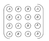
Substitutional disordered alloys. In such materials, there is an underlying lattice but each site of the lattice can be occupied by any constituents of the alloy as shown schematically in Fig. 15.1.
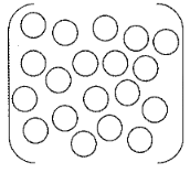
Amorphous systems. Such systems do not have any underlying lattice as shown schematically in Fig. 15.2. Amorphous Si, ordinary glass, and metallic glasses are some examples of such systems.
Theoretically, amorphous systems are more difficult to handle and will be discussed later in upcomming chapter . Here, we shall first try to develop methods for calculating the electronic structure of substitutional disordered alloys. This problem is best formulated in terms of Green’s function, which we discussed in chapter Section 14.1. For simplicity, we shall focus our discussion on random binary alloys. A random binary alloy has two components and each lattice site can be randomly occupied by any component with some probability. We shall denote an alloy of A and B atoms by \(A_xB_y\), where \(x\) and \(y\) denote the atomic concentrations of A and B atoms in the alloy. We shall start with the discussion of short and long-range order (LRO) in alloys in Section Section 15.2. Then, we discuss Green’s function for an ordered solid and for a substitutional impurity embedded in the ordered solid in Section Section 15.3. In Section Section 15.4, we shall come to the problem of disordered alloys and develop approximations such as CPA. In Section Section 15.5, we apply the theory to a tight-binding model. Since such a simple tight-binding model cannot be applied to realistic systems, we shall develop the formulation in the KKR framework using the muffin-tin model in Section Section 15.6. This theory is known as the KKR-CPA, which has been very successful in determining the electronic structure of realistic alloy systems and in making contact with experiments such as ARPES, 2D-ACAR, Compton, and optical experiments. Some examples of the KKR-CPA results for some alloys and comparison with experimental results will be given in Section Section 15.7. Finally, we shall discuss some theoretical attempts to go beyond the CPA and other recent developments in Section Section 15.8.
15.2 Short- and Long-Range Order
A random alloy, in which each site is occupied randomly by its constituent atoms, is an idealization. In general, there will be a deviation from a perfect random alloy and a real alloy may show some order. Depending on the length scales over which this order exists, we talk of short-range order (SRO) and long-range order (LRO). The SRO corresponds to the order that may exist at length scales of the order of nearest-neighbor distances whereas the LRO corresponds to the order that may exist over length scales approaching infinity. For example, in a crystalline solid, the atoms are arranged periodically and thus both LRO and SRO exist. In contrast, in an ideal gas, the atomic arrangement is totally random and therefore, both SRO and LRO are absent. In disordered alloys and amorphous materials, the LRO is absent but there may be some SRO. Similarly, in ferromagnets and antiferromagnets, the magnetic moments are aligned periodically, and, therefore, there is magnetic LRO.
The SRO can be characterized by an SRO parameter. For a disordered \(A_xB_y\) alloy, let \(p(A,B)\) be the probability of finding a B atom as a nearest neighbor of A atom. Warren-Cowley short-range parameter \(\boldsymbol{\alpha}\) for a nearest-neighbor pair is defined as
\[ \alpha = 1-p(A,B)/y \tag{15.1}\]
where \(y\) is the concentration of B atoms in the alloy. It can be seen from the above equation that \(\alpha=0\) represents a perfect random alloy as \(p(A,B)=y\) in this case. Similarly, \(\alpha<0\) when \(p(A,B)>y\), which means AB- and BA-type ordering is favored. Using similar logic, we can see that \(\alpha>0\) represents a system in which AA- and BB-type clustering is favored.
15.3 An Impurity in an Ordered Solid
Before we discuss Green’s function for an impurity in an ordered solid, we shall discuss how to obtain Green’s function for an ordered solid in the tight-binding representation.
15.3.1 Green’s function for an ordered solid
Using the procedure outlined in Chapter Section 14.1, we will construct Green’s function for a perfect solid, using a simple tight-binding model. In this case, the system is periodic and each site is identical. Let us assume a simple tight-binding Hamiltonian
\[ H = \sum_i |i\rangle \varepsilon_i \langle i| + \sum_{ij}' |i\rangle h_{ij}\langle j| \tag{15.2}\]
where \(|i\rangle\) and \(\langle j|\) denote Wannier functions centered at sites \(i\) and \(j\), \(\varepsilon_i\) are site energies, and \(h_{ij}\) are hopping matrix elements. Since each site is identical, \(\varepsilon_i=\varepsilon_0\). For simplicity, let us assume that
\[ \begin{aligned} h_{ij} &= h \quad \text{where } i \text{ and } j \text{ are nearest neighbors},\\ &=0 \quad \text{otherwise}. \end{aligned} \tag{15.3}\]
Since \(|i\rangle\) and \(\langle j|\) are orthonormal
\[ \langle i|j\rangle = \delta_{ij}. \tag{15.4}\]
The Wannier functions are related to Bloch functions \(|k\rangle\) by (see Equation Eq. 13.54)
\[ |k\rangle = \frac{1}{\sqrt{N}}\sum_i e^{i\vec k\cdot \vec R_i}|i\rangle \tag{15.5}\]
where \(\vec R_i\) is the position vector of site \(i\). The eigenvalues are given by (see Equation Eq. 13.48)
\[ \varepsilon_k = \varepsilon_0 + h\sum_i' e^{i\vec k\cdot \vec R_i} \tag{15.6}\]
where the prime over summation indicates that \(i=0\) term is excluded. In Equation Eq. 15.5, \(N\) is the total number of sites in the solid.
From Equation Eq. 15.5, we have
\[ \langle i|k\rangle = \frac{1}{\sqrt{N}}e^{i\vec k\cdot \vec R_i}. \tag{15.7}\]
Using Equation Eq. 14.14, we can write Green’s function as
\[ \begin{aligned} G_0(i,j,z)&=\langle i|G(z)|j\rangle\\ &=\sum_k\frac{\langle i|k\rangle\langle k|j\rangle}{z-\varepsilon_k}\\ &=\frac{1}{N}\sum_k\frac{e^{i\vec k\cdot(\vec R_i-\vec R_j)}}{z-\varepsilon_k}. \end{aligned} \tag{15.8}\]
If we put \(i=j\), we get
\[ \begin{aligned} G_0(i,i,z)&=\frac{1}{N}\sum_k\frac{1}{z-\varepsilon_k}\\ &=\frac{1}{N}\int \sum_k \frac{\delta(\varepsilon-\varepsilon_k)}{z-\varepsilon}\,d\varepsilon \end{aligned} \tag{15.9}\]
\[ =\int \frac{\rho(\varepsilon)}{z-\varepsilon}\,d\varepsilon. \tag{15.10}\]
Thus, if the DOS \(\rho(\varepsilon)\) is known, \(G_0(i,i,z)\) can be constructed using Equation Eq. 15.10. Alternatively, if \(G_0(i,i,z)\) is known, \(\rho(\varepsilon)\) can be calculated by taking the imaginary part of Equation Eq. 15.10 as we had seen in Chapter Section 14.1
\[ \rho(\varepsilon)=-\frac{1}{\pi}\operatorname{Im}G_0(i,i,\varepsilon^+). \tag{15.11}\]
15.3.2 Green’s function for a single impurity in a solid
Let us consider an impurity that is kept on a site \(i\) of an otherwise perfect solid. We assume that site energy at site \(i\) is
\[ \varepsilon_i=\varepsilon_0+\delta \tag{15.12}\]
where \(\varepsilon_0\) is the site energy at all other sites. The hopping elements between the nearest-neighboring sites are assumed to be \(h\). Let us write the Hamiltonian as
\[ H=H_0+H_1 \tag{15.13}\]
where
\[ H_0=\sum_i'|i\rangle\varepsilon_0\langle i|+\sum_{ij}'|i\rangle h\langle j| \tag{15.14}\]
and
\[ H_1=|i\rangle\delta\langle i|. \tag{15.15}\]
A prime over \(\sum\) in Equation Eq. 15.14 indicates that \(i=j\) is excluded and the sum is only over the nearest neighbors.
For Hamiltonian Eq. 15.14, we already know Green’s function \(G_0\) (see Equation Eq. 15.8). The Green function \(G\) for Hamiltonian Eq. 15.13 can be obtained by using Dyson’s equation (see Equation Eq. 14.41)
\[ \begin{aligned} G&=G_0+G_0H_1G\\ &=G_0+G_0H_1(G_0+G_0H_1G)\\ &=G_0+G_0H_1G_0+G_0H_1G_0H_1G_0+\cdots\\ &=G_0+G_0t_iG_0. \end{aligned} \tag{15.16}\]
where
\[ \begin{aligned} t_i&=H_1+H_1G_0H_1+\cdots\\ &=|i\rangle\delta\langle i|+|i\rangle\delta\langle i|G_0|i\rangle\delta\langle i|+\cdots\\ &=|i\rangle\left[\delta+\delta^2G_0(i,i,z)+\delta^3G_0^2(i,i,z)+\cdots\right]\langle i|\\ &=|i\rangle\frac{\delta}{1-\delta G_0(i,i,z)}\langle i|\\ &=|i\rangle\frac{\delta}{1-\delta F(z)}\langle i|. \end{aligned} \tag{15.17}\]
where
\[ F(z)=G_0(i,i,z). \tag{15.18}\]
Taking the matrix element of Equation Eq. 15.16, we get
\[ G(i,i,\varepsilon)=G_0(i,i,\varepsilon)+\frac{\delta G_0^2(i,i,\varepsilon)}{1-\delta G_0(i,i,\varepsilon)}. \tag{15.19}\]
Thus, we have found Green’s function for an impurity in a solid, from which we can find the DOS at site \(i\).
15.4 Disordered Alloy: General Theory
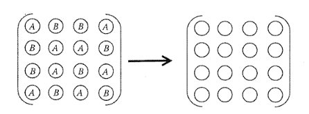
We assume a random binary alloy of say A and B atoms with concentration \(x\) and \(1-x\), respectively. This means each site can be occupied by A with probability \(x\) and by B with probability \(1-x\). As we have mentioned earlier, in a disordered alloy, there is no translational symmetry and as a result, Bloch’s theorem is not applicable. Thus, all the methods we have developed so far could not be applied to obtain the electronic structure of a disordered alloy. Since we are considering a substitutional disordered alloy, which has an underlying periodic lattice, we can make a simple approximation, that is, we replace the alloy by a periodic system of effective atoms as shown in Fig. 15.3. The effective atom can be chosen in many different ways:
- Virtual Crystal Approximation (VCA). We can assume that the effective atom has a potential, which is an average of the potentials of A and B atoms, that is
\[ v_{\mathrm{eff}}=xv_A+(1-x)v_B \tag{15.20}\]
where \(v_A\) and \(v_B\) are potentials of A and B atoms, respectively. This approximation is known as the VCA.
- Average t-Matrix Approximation (ATA). In this approximation, we assume that the \(t\)-matrix of the effective atom is an average of \(t_A\) and \(t_B\), the \(t\)-matrix of A and B atoms, respectively, that is
\[ \langle t\rangle=xt_A+yt_B, \tag{15.21}\]
where \(y=1-x\).
- Coherent Potential Approximation (CPA). In this approximation, the effective atom is chosen so that the average scattering from the effective atom is zero, that is, the average \(t\)-matrix from A or B atoms embedded in the effective medium is zero
\[ \langle t\rangle=xt_A+yt_B=0 \tag{15.22}\]
where \(t_A\) and \(t_B\) are the \(t\)-matrixes of A and B atoms embedded in the effective medium. This is known as CPA and is the best of the three approximations.
In the VCA, since the potential is real, Bloch’s states are still the solution of the problem, with infinite lifetimes. This is unphysical because due to the disorder in the system, Bloch’s states will scatter and will have a finite lifetime. However, in spite of this problem, it is sometimes used due to its simplicity. Now, we shall develop a theory of alloys using the ATA and CPA and derive the condition for finding the effective atom.
We assume that the one-electron Hamiltonian for the alloy \(A_xB_y\) can be written as
\[ H=H_0+V \tag{15.23}\]
where \(H_0\) is some suitably chosen periodic unperturbed Hamiltonian and \(V\) is the deviation from this periodic part. We assume that \(V\) can be written as the sum over site contributions
\[ V=\sum_i v_i \tag{15.24}\]
where \(i\) is the site index. For the binary \(A_xB_y\), \(v_i\) will take values \(v_A\) or \(v_B\) depending on whether \(i\) is occupied by A or B. Since for any value of \(x\), there will be a large number of possible configurations, \(H\) will be configuration dependent. However, we will be interested in configurational averages of physical quantities, such as charge density or DOS. For this purpose, we shall develop a theory in terms of the average Green’s function that can be directly related to these properties.
The average Green’s function \(G_{av}(z)\) can be written as
\[ G_{av}(z)=\langle G_c(z)\rangle \tag{15.25}\]
where \(\langle\cdots\rangle\) denotes the configurational average and \(G_c(z)\) is the configuration-dependent Green’s function
\[ G_c(z)=(z-H_c)^{-1}. \tag{15.26}\]
The average Green’s function can also be written in terms of self-energy \(\Sigma(z)\), which is periodic, that is
\[ \begin{aligned} G_{av}(z)&=(z-H)^{-1}\\ &=(z-H_0-\Sigma(z))^{-1}. \end{aligned} \tag{15.27}\]
We shall develop the approximation to find \(G_{av}(z)\) or alternatively \(\Sigma(z)\).
We first rewrite the Hamiltonian \(H\) by adding and subtracting a periodic potential
\[ \tilde V(z)=\sum_i \tilde v_i(z). \tag{15.28}\]
Thus,
\[ \begin{aligned} H&=H_0+V=H_0+\tilde V-\tilde V+V\\ &=\tilde H+U(z), \end{aligned} \tag{15.29}\]
where
\[ \tilde H=H_0+\tilde V \tag{15.30}\]
and
\[ U(z)=V-\tilde V=\sum_i\left(v_i-\tilde v_i(z)\right)=\sum_i u_i(z). \tag{15.31}\]
As we had seen in Section Section 14.3, \(G_c(z)\) can be expanded using Dyson’s equation
\[ \begin{aligned} G_c(z)&=(z-H_0-V)^{-1}\\ &=(z-\tilde H-U)^{-1}\\ &=\tilde G+\tilde GUG_c \end{aligned} \tag{15.32}\]
where
\[ \tilde G=(z-\tilde H)^{-1}=(z-H_0-\tilde V)^{-1}. \tag{15.33}\]
By repeatedly substituting Equation Eq. 15.32 for \(G_c\) on the right-hand side of Equation Eq. 15.32, we get an infinite series as
\[ \begin{aligned} G_c(z)&=\tilde G+\tilde G U\tilde G+\tilde G U\tilde G U\tilde G+\cdots\\ &=\tilde G+\tilde G(U+U\tilde G U+\cdots)\tilde G\\ &=\tilde G+\tilde G T\tilde G. \end{aligned} \tag{15.34}\]
where \(t\)-matrix \(T\) is
\[ \begin{aligned} T&=U+U\tilde G U+U\tilde G U\tilde G U+\cdots\\ &=\sum_i u_i+\sum_i u_i\tilde G\sum_j u_j+\cdots. \end{aligned} \tag{15.35}\]
Suppose, we have only one impurity at site \(i\), then \(u_j=0\) for \(j\ne i\) and \(T=t_i\), which can be written by using Equation Eq. 15.35 as
\[ \begin{aligned} t_i&=u_i+u_i\tilde G u_i+\cdots\\ &=u_i+u_i\tilde G(u_i+u_i\tilde G u_i+\cdots) \end{aligned} \tag{15.36}\]
\[ =t_i=u_i+u_i\tilde Gt_i. \tag{15.37}\]
where we used Equation Eq. 15.36 in writing Equation Eq. 15.37.
From Equation Eq. 15.37, we can get \(t_i\) in terms of \(u_i\) and \(\tilde G\) as
\[ t_i=(1-u_i\tilde G)^{-1}u_i. \tag{15.38}\]
Now, let us take the configurational average of Equation Eq. 15.34
\[ G_{av}=\langle G_c(z)\rangle=\tilde G+\tilde G\langle T\rangle\tilde G. \tag{15.39}\]
This is because \(\tilde G\) is a periodic function and is similar for each configuration. This can be rewritten as
\[ G_{av}=(1+\tilde G\langle T\rangle)\tilde G \tag{15.40}\]
or
\[ \begin{aligned} G_{av}^{-1}&=\tilde G^{-1}(1+\tilde G\langle T\rangle)^{-1}\\ &=\tilde G^{-1}(1+\tilde G\langle T\rangle-\tilde G\langle T\rangle)(1+\tilde G\langle T\rangle)^{-1}\\ &=\tilde G^{-1}(1-\tilde G\langle T\rangle(1+\tilde G\langle T\rangle)^{-1}). \end{aligned} \tag{15.41}\]
Using Equation Eq. 15.27, the self-energy can be written as
\[ \begin{aligned} \Sigma(z)&=z-H_0-G_{av}^{-1}\\ &=z-H_0-\tilde G^{-1}+\langle T\rangle(1+\tilde G\langle T\rangle)^{-1}\\ &=\tilde V+\langle T\rangle(1+\tilde G\langle T\rangle)^{-1} \end{aligned} \tag{15.42}\]
where we have used Equations Eq. 15.41 and Eq. 15.33.
Now, we return to Equation Eq. 15.35 and write it as
\[ T=\sum_i T_i \tag{15.43}\]
where
\[ \begin{aligned} T_i&=u_i+u_i\tilde G\sum_j u_j+u_i\tilde G\sum_j u_j\tilde G\sum_k u_k+\cdots\\ &=u_i+u_i\tilde G\left(\sum_j u_j+\sum_j u_j\tilde G\sum_k u_k+\cdots\right)\\ &=u_i+u_i\tilde G T\\ &=u_i(1+\tilde G T). \end{aligned} \tag{15.44}\]
where we have used Equation Eq. 15.35. Equation Eq. 15.44 can be further rewritten using Equation Eq. 15.43 as
\[ \begin{aligned} T_i&=u_i+u_i\tilde G\sum_jT_j\\ &=u_i+u_i\tilde G T_i+u_i\tilde G\sum_{j\ne i}T_j, \end{aligned} \tag{15.45}\]
or
\[ (1-u_i\tilde G)T_i=u_i+u_i\tilde G\sum_{j\ne i}T_j, \tag{15.46}\]
or
\[ \begin{aligned} T_i&=(1-u_i\tilde G)^{-1}u_i+(1-u_i\tilde G)^{-1}u_i\tilde G\sum_{j\ne i}T_j\\ &=t_i+t_i\tilde G\sum_{j\ne i}T_j, \end{aligned} \tag{15.47}\]
where we have used Equation Eq. 15.38. This can be rewritten by the repeated use of Equation Eq. 15.47 on the right-hand side
\[ T_i=t_i+t_i\tilde G\sum_{j\ne i}t_j+t_i\tilde G\sum_{j\ne i}t_j\tilde G\sum_{k\ne j}t_k+\cdots. \tag{15.48}\]
Substituting into Equation Eq. 15.43, we get
\[ T=\sum_i t_i+\sum_i t_i\tilde G\sum_{j\ne i}t_j+\sum_i t_i\tilde G\sum_{j\ne i}t_j\tilde G\sum_{k\ne j}t_k+\cdots. \tag{15.49}\]
The form of this expansion is interesting. We can see that the total scattering operator can be written as the sum of contributions coming from single-site scattering (first term), two-site scattering (second term), and so on. This is a multiple scattering expansion of \(T\) and, therefore, this theory is sometimes referred to as the multiple scattering theory.
Now, let us take the configurational average of Equation Eq. 15.43, that is
\[ \langle T\rangle=\sum_i\langle T_i\rangle \tag{15.50}\]
where using Equation Eq. 15.47, we get
\[ \begin{aligned} \langle T_i\rangle&=\left\langle t_i\left(1+\tilde G\sum_{j\ne i}T_j\right)\right\rangle\\ &=\langle t_i\rangle\left(1+\tilde G\sum_{j\ne i}\langle T_j\rangle\right)\\ &\quad + \left\langle (t_i-\langle t_i\rangle)\tilde G\sum_{j\ne i}(T_j-\langle T_j\rangle)\right\rangle. \end{aligned} \tag{15.51}\]
Now, we neglect the second term, that is, we neglect the correlations between sites \(j\) and \(i\). This is known as the single-site approximation (SSA). Such an approximation is not valid if there is short-range ordering or clustering in the system.
Now, using Equation Eq. 15.50, we write
\[ \langle T\rangle=\langle T_i\rangle+\sum_{j\ne i}\langle T_j\rangle \tag{15.52}\]
or
\[ \sum_{j\ne i}\langle T_j\rangle=\langle T\rangle-\langle T_i\rangle. \tag{15.53}\]
Now, substituting this into Equation Eq. 15.51 and neglecting the second term
\[ \langle T_i\rangle=\langle t_i\rangle(1+\tilde G\langle T\rangle-\tilde G\langle T_i\rangle), \tag{15.54}\]
or
\[ (1+\langle t_i\rangle\tilde G)\langle T_i\rangle=\langle t_i\rangle(1+\tilde G\langle T\rangle) \tag{15.55}\]
or
\[ \langle T_i\rangle=(1+\langle t_i\rangle\tilde G)^{-1}\langle t_i\rangle(1+\tilde G\langle T\rangle). \tag{15.56}\]
Now, we return to Equation Eq. 15.42 and write it as
\[ \begin{aligned} \Sigma(z)&=\sum_i\tilde v_i+\sum_i\langle T_i\rangle(1+\tilde G\langle T\rangle)^{-1}\\ &=\sum_i\sigma_i(z) \end{aligned} \tag{15.57}\]
where
\[ \begin{aligned} \sigma_i(z)&=\tilde v_i+\langle T_i\rangle(1+\tilde G\langle T\rangle)^{-1}\\ &=\tilde v_i+(1+\langle t_i\rangle\tilde G)^{-1}\langle t_i\rangle \end{aligned} \tag{15.58}\]
where we have used Equation Eq. 15.56.
Equation Eq. 15.58 suggests two ways of calculating self-energy \(\Sigma\).
- We can assume some periodic potential \(\tilde V\) and calculate \(\tilde G\) using Equation Eq. 15.33, so that \(\langle t_i\rangle\) can be calculated as
\[ \langle t_i\rangle=xt_A+yt_B \tag{15.59}\]
where \(t_A\) and \(t_B\) can be calculated using Equation Eq. 15.38. This approximation is known as the ATA and is not unique as it depends on the choice of \(\tilde V\).
- We can choose \(\tilde V\) such that \(\langle t_i\rangle=0\) so that the second term in Equation Eq. 15.58 is zero and
\[ \sigma_i(z)=\tilde v_i(z) \tag{15.60}\]
or
\[ \Sigma(z)=\tilde V(z). \tag{15.61}\]
That is, we choose the effective medium such that the average scattering from each site with respect to the effective medium is zero, that is
\[ \langle t_i\rangle=xt_A+yt_B=0. \tag{15.62}\]
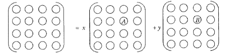
In other words, if we embed an A or B atom in the effective medium, the average scattering from this site is zero in accordance with Equation Eq. 15.62. This is known as CPA and is shown in Fig. 15.4. This is the best single-site approximation.
Let us write the CPA condition in terms of Green’s function. For this purpose, we fix the \(i=0\) site by putting an A atom and taking the configurational average of \(G_c\) (Equation Eq. 15.34) over all other sites
\[ \langle G_c\rangle_{0=A}=\tilde G+\tilde G\langle T\rangle_{0=A}\tilde G \tag{15.63}\]
where the symbol \(\langle\cdots\rangle_{0=A}\) represents restricted site averaging and means that configurational averaging has been taken with respect to all sites except \(i=0\) site.
Using Equation Eq. 15.43, we write
\[ \begin{aligned} \langle T\rangle_{0=A}&=\sum_i\langle T_i\rangle_{0=A}\\ &=\langle T_0\rangle_{0=A}+\sum_{i\ne0}\langle T_i\rangle_{0=A}. \end{aligned} \tag{15.64}\]
In the SSA, each site is surrounded by the effective medium; as a result, all fluctuations of the local environment are neglected. This implies that
\[ \langle T_i\rangle_{0=A}=\langle T_i\rangle\quad \text{for } i\ne0. \tag{15.65}\]
Also, by using Equation Eq. 15.47
\[ \begin{aligned} \langle T_0\rangle_{0=A}&=t_A+t_A\tilde G\sum_{i\ne0}\langle T_i\rangle_{0=A}\\ &=t_A\left(1+\tilde G\sum_{i\ne0}\langle T_i\rangle\right) \end{aligned} \tag{15.66}\]
where we have used Equation Eq. 15.65. Now, by using Equation Eq. 15.51 (neglecting the last term of Equation Eq. 15.51), this can be written as
\[ \langle T_0\rangle_{0=A}=t_A\langle t_0\rangle^{-1}\langle T_0\rangle. \tag{15.67}\]
Thus, we can write Equation Eq. 15.64 as
\[ \begin{aligned} \langle T_0\rangle_{0=A}&=t_A\langle t_0\rangle^{-1}\langle T_0\rangle+\sum_{i\ne0}\langle T_i\rangle\\ &=t_A\langle t_0\rangle^{-1}\langle T_0\rangle+\langle T\rangle-\langle T_0\rangle\\ &=\langle T\rangle+(t_A\langle t_0\rangle^{-1}-1)\langle T_0\rangle\\ &=\langle T\rangle+(t_A-\langle t_0\rangle)\langle t_0\rangle^{-1}\langle T_0\rangle\\ &=\langle T\rangle+(t_A-xt_A-yt_B)\langle t_0\rangle^{-1}\langle T_0\rangle\\ &=\langle T\rangle+y(t_A-t_B)\langle t_0\rangle^{-1}\langle T_0\rangle. \end{aligned} \tag{15.68}\]
where \(y=1-x\). Similarly, it can be shown that
\[ \langle T\rangle_{0=B}=\langle T\rangle+x(t_B-t_A)\langle t_0\rangle^{-1}\langle T_0\rangle. \tag{15.69}\]
Equations Eq. 15.68 and Eq. 15.69 imply that
\[ x\langle T\rangle_{0=A}+y\langle T\rangle_{0=B}=\langle T\rangle. \tag{15.70}\]
As a result from Equation Eq. 15.63
\[ \begin{aligned} x\langle G_c\rangle_{0=A}+y\langle G_c\rangle_{0=B}&=\tilde G+\tilde G(x\langle T\rangle_{0=A}+y\langle T\rangle_{0=B})\tilde G\\ &=\tilde G+\tilde G\langle T\rangle\tilde G\\ &=G_{av}. \end{aligned} \tag{15.71}\]
Equation Eq. 15.71 is another way of writing CPA conditions that we shall use later.
15.5 Application to the Single Band Tight-Binding Model of Disordered Alloy
We assume a tight-binding model for the disordered alloy \(A_xB_{1-x}\), described by the Hamiltonian \(H\)
\[ H=\sum_i |i\rangle\varepsilon_i\langle i|+\sum_{ij}'|i\rangle h\langle j|. \tag{15.72}\]
Here, all \(\varepsilon_i\)’s are not equal but take values, \(\varepsilon_A\) or \(\varepsilon_B\) depending on whether the site is occupied by atom A or B. In Equation Eq. 15.72, \(h\) is the hopping matrix element between the nearest-neighbor sites and is assumed to be similar irrespective of the disorder. In other words, we ignore the off-diagonal disorder in \(H\).
For convenience, we shall express \(\varepsilon_A\) and \(\varepsilon_B\) in units of \(\omega\) and define the zero of energy such that
\[ \varepsilon_A=\frac{1}{2}\omega\delta \quad \text{and} \quad \varepsilon_B=-\frac{1}{2}\omega\delta \tag{15.73}\]
where
\[ \delta=\frac{\varepsilon_A-\varepsilon_B}{\omega}. \tag{15.74}\]
\(\omega\) is a scaling factor, which for convenience will be chosen equal to unity.
We choose
\[ \tilde H=H_0+\sum_i |i\rangle\tilde V\langle i| \tag{15.75}\]
and
\[ H_{eff}=H_0+\sum_i |i\rangle\Sigma\langle i| \tag{15.76}\]
where \(H_0\) is the Hamiltonian corresponding to a simple tight-binding model of a simple cubic lattice, \(\tilde H\) the Hamiltonian of a periodic system with potential \(\tilde V\) at each site, and \(H_{eff}\) effective Hamiltonian for the alloy with self-energy \(\Sigma\) at each site. Note that \(\tilde V\) and \(\Sigma\) are simply numbers and not operators as in the previous section.
Now, we shall use ATA and CPA conditions (Equations Eq. 15.59 and Eq. 15.61), to obtain self-energy \(\Sigma(z)\). For this, we have to know \(\langle t_i\rangle\), which we can find using Equation Eq. 15.17.
\[ \begin{aligned} \langle t_i\rangle&=xt_A+yt_B\\ &=|i\rangle\left[x\frac{(\varepsilon_A-\tilde V)}{1-(\varepsilon_A-\tilde V)\tilde F}+y\frac{(\varepsilon_B-\tilde V)}{1-(\varepsilon_B-\tilde V)\tilde F}\right]\langle i| \end{aligned} \tag{15.77}\]
where
\[ \begin{aligned} \tilde F&=\tilde G(i,i,z)\\ &=G_0(i,i,z-\tilde V). \end{aligned} \tag{15.78}\]
This is because \(\tilde H\) differs from \(H_0\) only by a constant \(\tilde V\). Substituting Equation Eq. 15.77 into Equation Eq. 15.58 of the previous section, we get the self-energy \(\Sigma(z)\) in ATA.
The self-energy in the CPA is obtained by substituting \(\tilde V=\Sigma\) into Equation Eq. 15.77 and setting \(\langle t_i\rangle=0\). This gives
\[ \Sigma=x\varepsilon_A+(1-x)\varepsilon_B-(\varepsilon_A-\Sigma)\tilde F(\varepsilon_B-\Sigma). \tag{15.79}\]
Using this equation, \(\Sigma\) can be obtained by using an iterative procedure. Once \(\Sigma\) is known, one obtains the DOS
\[ \begin{aligned} \rho(\varepsilon)&=-\frac{1}{\pi}\operatorname{Im}G(i,i,\varepsilon)\\ &=-\frac{1}{\pi}\operatorname{Im}G_0(i,i,\varepsilon-\Sigma). \end{aligned} \tag{15.80}\]
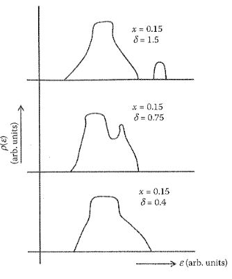
The DOS for this simple cubic tight-binding model is schematically shown in Fig. 15.5 for various values of \(\delta\) and \(x=0.15\) (Ehrenreich and Schwartz 1976). We see that for \(\delta=0.4\), the DOS gets somewhat distorted but looks similar to the DOS of the ordered material (see Figure 5.9) except that there are no sharp features corresponding to van Hove singularities. For \(\delta=0.75\), there is appearance of a structure in the upper part of the DOS. For \(\delta=1.5\), something very drastic happens and the DOS splits into two, with an energy gap in between. Thus, by increasing \(\delta\) beyond 1.0, the single \(s\) band splits into two bands that is an important effect of the disorder. This range of \(\delta>1\) is called the split band regime. This is similar to what happens in the Hubbard model for large electron-electron repulsion U. This is not surprising because it is possible to map the Hubbard model onto the tight-binding alloy model for \(x=y=(1/2)\) (Velicky et al. 1968).
15.6 Muffin-Tin Model: KKR-CPA
The single band tight-binding model of a disordered alloy discussed in Section Section 15.5 is not applicable to real systems such as Cu-Zn alloy because a real system has many bands. One can generalize this model to many bands, but then it has too many parameters. What we would like to develop is a parameter-free theory of the electronic structure of a disordered alloy similar to the one we have already discussed for the periodic solids. We shall see that this is possible if we use muffin-tin model of the alloy and apply the idea of the CPA developed in Section Section 15.4. In Chapter Section 14.1, we developed the KKR method for periodic solids using the muffin-tin model and Green’s function. For disordered alloys, we shall develop the KKR-CPA method that combines the ideas of the KKR method and the CPA. Within the DFT, this gives rise to a first-principles theory of the electronic structure of disordered alloys. As the algebra involved in developing the theory is quite complicated, we shall highlight the important points and give only the outline of the derivation.
As we had seen in Chapter Section 14.1, a muffin-tin potential is spherically symmetric and finite within a radius \(r_m\), called muffin-tin radius and is zero outside it. Thus, for a disordered \(A_xB_{1-x}\) alloy, there will be two types of muffin-tin potentials, \(v_A(r)\) and \(v_B(r)\) representing A and B atoms. We assume that the potentials centered on different sites do not overlap. For a particular configuration of the alloy, one-electron Hamiltonian can be written as
\[ H(\vec r)=H_0(\vec r)+V(\vec r) \tag{15.81}\]
where \(H_0(\vec r)\) is the free-electron Hamiltonian and \(V(\vec r)\) can be decomposed as
\[ V(\vec r)=\sum_i v_i(\vec r_i) \tag{15.82}\]
where the sum is over all sites and \(\vec r_i=\vec r-\vec R_i\), \(\vec R_i\) being the position vector of the \(i\)th site. \(v_i(\vec r_i)\) is the muffin-tin potential centered at \(\vec R_i\) and is equal to \(v_A(\vec r_i)\) or \(v_B(\vec r_i)\) depending on whether \(i\) is occupied by an A or B atom.
As in Chapter Section 14.1, we shall use the abstract vector space and use the convention that
\[ H(\vec r)=\langle \vec r|H|\vec r\rangle \tag{15.83}\]
where
\[ H=H_0+V. \tag{15.84}\]
Green’s function for this configuration in the abstract vector space can be written as
\[ G_c(\varepsilon)=(\varepsilon+i0-H)^{-1}. \tag{15.85}\]
We are interested in \(G_{av}(\varepsilon)\), the average of \(G_c\) over all configurations of the alloy, that is
\[ G_{av}=\langle G_c(\varepsilon)\rangle=\left\langle(\varepsilon+i0-H)^{-1}\right\rangle. \tag{15.86}\]
As we had seen in Section Section 15.4, \(G_c(\varepsilon)\) can be expanded as
\[ G_c(\varepsilon)=G_0(\varepsilon)+G_0TG_0. \tag{15.87}\]
\(T\) is given by
\[ T=\sum_i t_i+\sum_i t_iG_0\sum_{j\ne i}t_j+\cdots \tag{15.88}\]
where \(t_i\) is atomic \(t\)-matrix given by
\[ t_i=v_i(1-G_0v_i)^{-1}. \tag{15.89}\]
Equation Eq. 15.88 is an infinite series, which can be written in a closed form if we decompose \(T\) as
\[ T=\sum_{ij}T_{ij}. \tag{15.90}\]
Then \(T_{ij}\) satisfies the equation
\[ T_{ij}=t_i\delta_{ij}+t_iG_0\sum_{k\ne i}T_{kj}. \tag{15.91}\]
This can be checked by substituting Equation Eq. 15.91 into Equation Eq. 15.90 repeatedly that gives us Equation Eq. 15.88. \(T_{ij}\) are called path operators and describe all possible scattering processes beginning at site \(i\) and ending at site \(j\) (Gyorffy 1972). Equation Eq. 15.91 is exact and represents infinite coupled operator equations for \(T_{ij}\), which in general cannot be solved. The use of nonoverlapping muffin-tin potentials greatly simplifies the algebra making these equations solvable. Because of the spherical symmetry of the muffin-tin potential, the use of angular momentum representation is particularly convenient and simplifies the algebra. The matrix elements of \(t_i\) and \(T_{ij}\) in the coordinate representation can be expanded as
\[ \begin{aligned} \langle\vec r|t_i|\vec r'\rangle&=t_i(\vec r_i,\vec r_i')\\ &=\sum_LY_L(\hat r_i)t_i^\ell(r_i,r_i')Y_L(\hat r_i') \end{aligned} \tag{15.92}\]
\[ \begin{aligned} \langle\vec r|T_{ij}|\vec r'\rangle&=T_{ij}(\vec r_i,\vec r_j')\\ &=\sum_{LL'}Y_L(\hat r_i)T_{ij}^{LL'}(\vec r_i,\vec r_j')Y_{L'}(\hat r_j') \end{aligned} \tag{15.93}\]
where \(L\) is a composite index \((\ell,m)\) and \(Y_L\) are spherical harmonics. The Fourier transform of \(t_i(\vec r_i,\vec r_i')\) can be written as
\[ t_i(\vec k,\vec k')=\iint e^{-i\vec k\cdot\vec r_i}t_i(\vec r_i,\vec r_i')e^{i\vec k'\cdot\vec r_i'}d^3r_i\,d^3r_i'. \tag{15.94}\]
The \(k=k'=\kappa=\sqrt{2\varepsilon}\) (in a.u.) matrix element, called the energy shell matrix element, can be easily evaluated in terms of the phase shift \(\delta_i^\ell(\kappa)\) of potential \(v_i(r)\)
\[ t_i^\ell(\kappa,\kappa)=t_i^\ell(\kappa)=-\frac{1}{\kappa}e^{i\delta_i^\ell}\sin\delta_i^\ell. \tag{15.95}\]
It turns out that most of the properties of interest such as the DOS can be expressed in terms of only the energy shell matrix elements of \(t_i\) and \(T_{ij}\) operators. Thus, Equation Eq. 15.91 reduces to the following system of linear algebraic equations in terms of energy shell matrix elements \(t_i^\ell(\kappa)\) and \(T_{ij}^{LL'}(\kappa)\)
\[ T_{ij}^{LL'}(\kappa)=t_i^\ell(\kappa)\delta_{ij}\delta_{LL'}+t_i^\ell(\kappa)\sum_{pL''}B_{ip}^{LL''}(\kappa)T_{pj}^{L''L'}(\kappa) \tag{15.96}\]
where \(B_{ip}^{LL'}(\kappa)\) is off-diagonal, that is, zero for \(i=p\). It is related to the Fourier transform of the usual KKR structure constants and depends only on the lattice structure (Ehrenreich and Schwartz 1976). The solution of Equation Eq. 15.96 is
\[ T^{LL'}(\kappa)=\left[(t^\ell(\kappa))^{-1}-B\right]^{-1}_{LL'}. \tag{15.97}\]
Now, let us find the configuration-dependent Green’s function \(G_c\) in the coordinate representation. It is more convenient to express \(G_c(\vec r,\vec r',\varepsilon)\) in terms of regular and irregular solutions \(Z_i^\ell(\vec r,\varepsilon)\) and \(J_i^\ell(\vec r,\varepsilon)\) of the Schrödinger equation for an isolated potential \(v_i(r)\) (Faulkner and Stocks 1980). \(Z_i^\ell(\vec r,\varepsilon)\) and \(J_i^\ell(\vec r,\varepsilon)\) are normalized such that for \(r\ge r_m\),
\[ Z_i^\ell(\vec r,\varepsilon)=\kappa Y_L(\hat r)\left[n_\ell(\kappa r)-\cot\delta_i^\ell j_\ell(\kappa r)\right] \tag{15.98}\]
and
\[ J_i^\ell(\vec r,\varepsilon)=Y_L(\hat r)j_\ell(\kappa r) \tag{15.99}\]
where \(j_\ell\) and \(n_\ell\) are spherical Bessel and Neumann functions, respectively. In terms of these functions, \(G_c(\vec r,\vec r',\varepsilon)\) can be expressed as
\[ G_c(\vec r,\vec r',\varepsilon)=\sum_{LL'}Z_i^L(\vec r,\varepsilon)T_{ij}^{LL'}(\kappa)Z_j^{L'}(\vec r',\varepsilon)-\sum_LZ_i^L(\vec r_<,\varepsilon)J_i^L(\vec r_>,\varepsilon). \tag{15.100}\]
Equation Eq. 15.100 is exact within the muffin-tin approximation and can be used to evaluate Green’s function for a finite system such as a cluster of atoms. For infinite systems, such as the disordered alloy, this is not possible as it requires inversion of a matrix of infinite size in Equation Eq. 15.97 and then averages over all configurations. Therefore, to make further progress, we resort to the CPA, which in this context is known as the KKR-CPA. As we had seen in Section Section 15.4, in this approximation, the alloy \(A_xB_{1-x}\) is replaced by a periodic effective medium, which is determined by the requirement that if a particular site say \(i=0\) site is replaced by an A or B atom, the average scattering from this site with respect to the medium is zero, that is
\[ x\langle G_c\rangle_{0=A}+y\langle G_c\rangle_{0=B}=\langle G_c\rangle. \tag{15.101}\]
If \(t_A\) and \(t_B\) represent the energy shell matrix element of the atomic \(t\)-matrix for A and B atoms, respectively and \(t_c\) represents the energy shell matrix element of the effective atom, then Equation Eq. 15.101 gives the KKR-CPA condition as
\[ t_c^{-1}=xt_A^{-1}+(1-x)t_B^{-1}+(t_A^{-1}-t_c^{-1})T_{00}^c(t_B^{-1}-t_c^{-1}) \tag{15.102}\]
where
\[ T_{00}^c=\frac{1}{N}\sum_{\vec k}\left[t_c^{-1}-B(\vec k,\varepsilon)\right]^{-1} \tag{15.103}\]
where \(N\) is the number of unit cells in the alloy. The energy shell matrix element \(t_c\) can be obtained by solving Equation Eq. 15.102 self-consistently. This is a nontrivial task as it involves Brillouin zone integration at each step through Equation Eq. 15.103. This was a big hurdle in the early stage that was overcome by using a simple method of integration called special direction method (Bansil 1975, Prasad and Bansil 1980). Although this method is computationally very efficient, it is not as accurate as the tetrahedron method that was later developed for disordered alloys (Kaprzyk and Mijnarends 1986).
For the charge self-consistent calculation, we need charge densities in A and B cells. These are obtained from the restricted site averages of Green’s function in Equation Eq. 15.100 that we shall denote by \(\langle G(\vec r,\vec r',\varepsilon)\rangle_{A(B)}\). Let \(\rho_{A(B)}(\vec r)\) denote the charge density associated with an A(B) cell that can be written as
\[ \rho_{A(B)}(\vec r)=-\frac{1}{\pi}\int^{\varepsilon_F}\operatorname{Im}\langle G(\vec r,\vec r,\varepsilon)\rangle_{A(B)}d\varepsilon \tag{15.104}\]
where \(\varepsilon_F\) is the Fermi energy. Note that we have assumed the system to be at absolute zero temperature. The integration in Equation Eq. 15.104 is along the real energy that takes much computer time. This problem was addressed by Zeller et al. (1982), who used the complex energy method to speed up the calculation. This also makes the \(k\)-space integration faster because the integrand becomes smoother for the complex energies.
The Fermi energy \(\varepsilon_F\) is calculated by requiring that the integrated density of states (IDOS) at the Fermi energy gives the average number of electrons in the cell. Generally, the IDOS is calculated from Lloyd’s formula given by
\[ \begin{aligned} N(\varepsilon)&=N_0(\varepsilon)+\frac{2}{\pi}\operatorname{Im}\left[x\ln\left\|t_c^{-1}-t_B^{-1}\right\|+y\ln\left\|t_c^{-1}-t_A^{-1}\right\|\right]\\ &\quad -\frac{2}{\pi N}\sum_{\vec k}\operatorname{Im}\ln\left\|t_c^{-1}-B(\vec k,\varepsilon)\right\| \end{aligned} \tag{15.105}\]
where \(N(\varepsilon)\) is the IDOS for the alloy and \(N_0(\varepsilon)\) is the IDOS for the free electrons. This formula is very convenient to use but sometimes gives unphysical jumps. This problem was pursued by Kaprzyk and Bansil (1990) who derived a generalized Lloyd formula that does not give unphysical jumps.
The average DOS can be calculated by differentiating IDOS \(N(\varepsilon)\) from Equation Eq. 15.105. But the component DOS is calculated from the restricted site-averaged Green’s function \(\langle G(\vec r,\vec r',\varepsilon)\rangle_{A(B)}\) as
\[ \rho_{A(B)}(\varepsilon)=-\frac{1}{\pi}\int \operatorname{Im}\langle G(\vec r,\vec r,\varepsilon)\rangle_{A(B)}d^3r \tag{15.106}\]
where the integration is over the unit cell.
The charge self-consistent KKR-CPA calculation is carried out in the following steps:
We start with some initial guess for the potentials \(v_A\) and \(v_B\) and solve the KKR-CPA Equation Eq. 15.102.
The new charge densities in A and B cells are then obtained using Equation Eq. 15.104.
New potentials \(v_{A(B)}\) in A and B cells are obtained from these charge densities.
The whole procedure is iterated until the self-consistency is achieved. This means that, at the final step, the input and output potentials are the same within some tolerance. We note that the converged potentials do not depend on the initial choice of the potentials \(v_A\) and \(v_B\) and hence, the final results for the band structure, DOS, and so on are also independent of the initial choice of the potentials.
We see that the KKR-CPA theory does not involve any adjustable parameter and therefore is a first-principles theory of the random alloys. It shows correct limiting behavior, that is, in \(x\to0\) limit, it reduces to the standard KKR band theory discussed in Chapter Section 14.1. It also describes the impurity limit correctly. Thus, it is a very general theory that can treat pure metals, single impurity, and concentrated alloys at the same level. In the following section, we discuss some applications of the KKR-CPA.
15.7 Application of the KKR-CPA: Some Examples
The KKR-CPA method has been applied to a large number of alloy systems. To illustrate some salient features of the KKR-CPA, we present some representative results. For more applications to many other systems, we refer to the review articles given at the end of this chapter.
15.7.1 Density of States
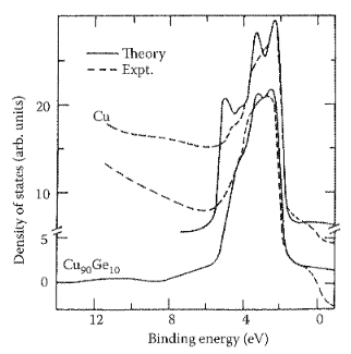
As an example of the average DOS of a disordered alloy, we show in Fig. 15.6 the KKR-CPA average DOS for \(\mathrm{Cu}_{0.9}\mathrm{Ge}_{0.1}\) alloy (Prasad and Bansil 1982). The DOS for pure Cu is also shown in the figure along with the experimental results by Norris and Williams (1978). We note that the experimental results are in reasonably good agreement with the theoretical results. We see that there is a large broadening of the structure due to alloying at the top and bottom of the Cu-\(d\)-band (i.e., around 2 and 5 eV below 0) that is correctly predicted by the theory. Further, there is a small bump in the energy range of 10-12 eV below 0 in the KKR-CPA results for the alloy. This bump arises due to a new band in the alloy band structure that can be attributed to Ge in the alloy. This is similar to what we saw in the tight-binding model of the disordered alloy when we increased \(\delta\) beyond 1 in Section Section 15.5. This means that the new band arises because \(s\)-\(p\) states of Cu and Ge experience a large disorder. We see this new band in Fig. 15.7 as discussed below.
15.7.2 Complex Energy Bands
The concept of energy bands is an important concept in the theory of ordered solids that is very useful in interpreting various experimental results. This concept can be generalized to disordered alloys but now the energy bands become complex. To see this, recall that in the KKR theory of ordered solids that we discussed in Chapter Section 14.1, the energy bands are given by the KKR equation that can be written as (Exercise 8.4)
\[ \left\|\left|t^{-1}-B(\vec k,\varepsilon)\right|\right\|=0. \tag{15.107}\]
It turns out that for disordered alloys, one gets a similar equation for the energy bands (Bansil 1978, 1979a,b, 1987)
\[ \left\|\left|t_c^{-1}-B(\vec k,\varepsilon)\right|\right\|=0. \tag{15.108}\]
This equation reduces to Equation Eq. 15.107 in the limit of pure A(B) material, that is, when \(t_c=t_{A(B)}\). This equation can be solved in two ways: (i) first fix \(\vec k\) and then look for the root of the determinant to obtain \(\varepsilon_i\) and (ii) first fix \(\varepsilon\) and then find the roots of the determinant to find constant energy surfaces in \(\vec k\) space. To obtain energy bands, one uses the first method whereas to obtain Fermi surface, one uses the second method. First, let us focus on \(\varepsilon\) versus \(\vec k\) curve. We know that \(\varepsilon_i\) are real for the ordered material but interestingly turn out to be complex in alloys. This is because of disorder scattering that makes determinant Eq. 15.108 to be complex; as a result, it has roots at complex energies if we assume \(\vec k\) to be real. Thus, the imaginary part of \(\varepsilon_i\) can be associated with the disorder scattering and is an important effect of disorder. It makes the alloy bands fuzzy and therefore is also known as disorder smearing.
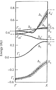
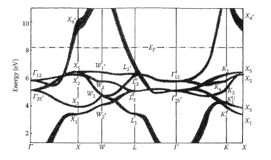
It is interesting to note that in Chapters Section 12.1 through Section 14.1, the concept of energy bands and energy gaps emerged from translational symmetry. The theory of disordered alloys tells us that it may not be necessarily the case. The disordered alloys can have well-defined bands, provided the separation between them is much larger than their disorder smearing. To see that this is indeed the case, we shall show energy bands of disordered \(\mathrm{Cu}_{0.9}\mathrm{Ge}_{0.1}\) and \(\mathrm{Cu}_{0.9}\mathrm{Al}_{0.1}\) alloys. In Fig. 15.7, we show the complex energy bands for \(\mathrm{Cu}_{0.9}\mathrm{Ge}_{0.1}\) alloy along \(\Gamma X\) direction (Prasad and Bansil 1982). The dark line represents the real part of the energy and the shading around the bands represents the disorder smearing. We clearly see that there are well-defined bands and the disorder smearing is much smaller than the band separations. We see that, in general, the disorder smearing changes from band to band and could be \(\vec k\) dependent. Most importantly, we see that as a result of alloying a new band around \(-0.2\) Ry due to Ge impurities appears below Cu band structure. As we had discussed above, this band appears because of the large disorder in Cu and Ge \(s\)-\(p\) states. The band structure of Cu-Ge alloys was measured by ARPES experiment and was found to be in good agreement with the KKR-CPA results (Bansil et al. 1984). In Fig. 15.8, we show the complex energy bands for disordered \(\mathrm{Cu}_{0.9}\mathrm{Al}_{0.1}\) alloy (Asonen et al. 1982). In the figure, the disorder smearing of a band is shown by the vertical width of the band. We clearly see that there are well-defined bands and the disorder smearing is much smaller than the band separations as was the case with Cu-Ge alloy. We see that the disorder smearing changes from band to band and is \(\vec k\) dependent. We further note that the band structure of the \(\mathrm{Cu}_{0.9}\mathrm{Al}_{0.1}\) alloy looks similar to the band structure of copper shown in Figure 4.11 except that the bands in the alloy are smeared. In Fig. 15.8, the \(d\) bands lie in the range of 4-7 eV whereas the band near the Fermi energy largely has \(s\)-\(p\) character. We also see that the disorder smearing in \(s\)-\(p\) bands is larger than that of the \(d\) bands. This is because the \(d\) states see much less disorder as there are no \(d\) electrons in Al. The band structure of Fig. 15.8 was found to be in good agreement with ARPES results.
The energy bands and band gaps in disordered alloys can be probed by a variety of experimental techniques such as ARPES, optical absorption, differential reflectivity, and piezoreflectance techniques. These experiments have confirmed the existence of energy bands and energy gaps in disordered alloys. For example, using ARPES, the alloy energy bands have been measured for many alloys and are found in good agreement with the KKR-CPA results (see, e.g., Bansil and Pessa 1983, Bansil et al. 1984, Asonen et al. 1982). Rao et al. (1983) calculated the composition dependence of various gaps using the KKR-CPA for many Cu-based alloy systems and found it in good agreement with the experimental results. As was the case for ordered materials, the complex energy band structure of a disordered alloy has been found to be very useful in interpreting various experiments. It gives deeper insight, helps understand the formation of new bands, and how the bands of a disordered alloy evolve as a function of alloying.
15.7.3 Fermi Surface
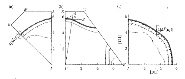
We saw in Section Section 15.7.2 that the disordered alloys can have well-defined bands. If the band intersecting the Fermi energy is well defined, the disordered alloy should have a well-defined Fermi surface. Fermi surface is obtained by fixing \(\varepsilon\) and looking for the roots of determinant Eq. 15.108. Now, the energy \(\varepsilon\) is real; therefore, the roots of Equation Eq. 15.108 occur at complex values of \(\vec k\), whose imaginary part represents disorder scattering and is called disorder smearing. Note that the disorder smearing of the Fermi surface depends on the direction of \(\vec k\). As a result of disorder smearing, the Fermi surface of a disordered alloy is fuzzy and is not sharp as is the case for pure metals. As an example of the alloy Fermi surface in Fig. 15.9, we show few typical cross-sections of the Fermi surface of \(\mathrm{Cu}_{0.7}\mathrm{Zn}_{0.3}\) alloy obtained by using the KKR-CPA (Prasad et al. 1981). We see that the alloy Fermi surface is fuzzy as opposed to the Cu Fermi surface that is also shown in Fig. 15.9 and is sharp. In the figure, the theoretical results have been compared with the results obtained from two-dimensional angular correlation of positron annihilation radiation (2D-ACAR) experiment and are found to be in good accord. The 2D-ACAR technique has been used to obtain Fermi surface dimensions for several disordered alloys such as Cu-Zn, Cu-Pd, Nb-Mo, and Li-Mg (see, e.g., Prasad et al. 1981, Matsumoto et al. 2001, Rajput et al. 1993, 1996). It has been found that the KKR-CPA does extremely well in predicting the Fermi surfaces of disordered alloys. Also, experiments have established that, in general, concentrated metallic alloys do have well-defined Fermi surfaces.
15.8 Beyond CPA
As we have already mentioned, the CPA is a single-site approximation and, therefore, neglects correlations between the two atoms in the alloy. In many alloy systems, such as CuPd and CuNi that show short-range ordering or clustering, such correlations cannot be neglected and thus cannot be handled by using the CPA. To deal with such local environmental effects, one has to go beyond such single-site schemes such as the CPA and develop theories using multisite or cluster approximations. However, this problem turned out to be extremely difficult. Here, briefly we shall review some attempts to go beyond the CPA.
It turns out that the CPA has many good features such as it always yields positive DOS. In other words, the CPA Green’s function is always analytic in the upper half of the complex energy plane. Also, it preserves the translational invariance and the point-group symmetry of the underlying lattice. It was found that a simple cluster generalization of the CPA does not preserve these properties leading to unphysical results such as negative DOS (Butler 1973, Nickel and Butler 1973). One of the first successful attempts that preserves the above-mentioned properties was due to Mills and Ratanavararaksa (1978) who developed a traveling cluster approximation using a diagrammatic technique. Mookerjee and coworkers (Mookerjee 1973, Bishop and Mookerjee 1974, Razee et al. 1991) developed a CCPA using the augmented space formalism that also preserves the analytic properties of the averaged Green’s function. This method was generalized to the muffin-tin model and the KKR-CCPA scheme was developed (Razee et al. 1990, Razee and Prasad 1992, 1993a,b, Mookerjee and Prasad 1993). Recently, this method has been applied to CuZn alloys by Rahaman and Mookerjee (2009). Mookerjee and coworkers also developed a method that incorporates environmental effects using the recursion scheme in the augmented space (Saha et al. 1994). More recently, Rowland and coworkers have developed an NLCPA, which also preserves the analytical properties and translational invariance of the underlying lattice. Rowland and coworkers have also applied it to the muffin-tin model and developed KKR-NLCPA (Rowlands 2009). Also, Skriver and Ruban have developed an LSGF method that is also analytic and computationally very efficient (Ruban and Abrikosov 2008). For details, we refer to the original papers and review articles.
15.9 Exercises
Derive the CPA condition Eq. 15.79 for a single band tight-binding model of a disordered alloy.
Calculate the DOS for a binary random alloy with a cubic lattice using the CPA and the single band tight-binding model. Compare your results with the results of Fig. 15.5.
Calculate the DOS for a binary random alloy when the DOS corresponding to the Hamiltonian \(H_0\) in Equation Eq. 15.76 is given in the form
\[ \rho_0(\varepsilon)=\left(\frac{2}{\pi w^2}\right)(w^2-\varepsilon^2)\quad \text{for } |\varepsilon|\le w \tag{15.109}\]
\[ \rho_0(\varepsilon)=0,\quad \text{for } |\varepsilon|\ge w. \tag{15.110}\]
Do you get the same trend as in Exercise 8.2 by changing \(\delta\) and \(x\)?
(Hint: see the paper by Velicky et al. (1968).)
Calculate the DOS for disordered \(\mathrm{Cu}_{0.9}\mathrm{Ge}_{0.1}\) alloy using the KKR-CPA method. Compare your result with Fig. 15.6. You may use the KKR-CPA code mentioned in Appendix A.
Calculate the DOS for the disordered \(\mathrm{Cu}_{0.7}\mathrm{Zn}_{0.3}\) alloy using the KKR-CPA method. You may use the KKR-CPA code mentioned in Appendix A.
Calculate the Fermi surface for disordered \(\mathrm{Cu}_{0.7}\mathrm{Zn}_{0.3}\) alloy using the KKR-CPA method. Compare your results with Fig. 15.9. You may use the KKR-CPA code mentioned in Appendix A.
15.10 Further Reading
Bansil A. 1987. Modern band theory of disordered alloys. Lect. Notes Phys. 283: 273-298. Berlin: Springer.
Faulkner J. S. 1982. Modern theory of alloys. Progress in Material Science, 27:1-187.
Prasad R. 1994. KKR approach to random alloys. In Methods of Electronic Structure Calculations eds., Andersen O. K., Kumar V., and Mookerjee A. pp. 211-230. Singapore: World Scientific.