10 Density Functional Theory
10.1 Introduction
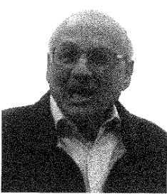
Until now we have been trying to solve the many-body problem by approximating the many-body wave function such as in Hartree or Hartree–Fock (H–F) methods. Since the many-body wave function involves the coordinates of all the electrons, it is a function of \(3N\) variables, where \(N\) is the number of electrons. Obviously, such an approach is complex and numerically very demanding. It would be much simpler if the electronic system could be described in terms of electron density \(n(\vec{r})\), which is a function of only three variables (e.g., \(x\), \(y\), \(z\)). A firm and exact theoretical foundation for such description was provided by Hohenberg and Kohn in 1964 and is known as the density functional theory (DFT). We shall see that in the local density approximation (LDA) it is as simple as the Hartree theory but gives much better results than that given by the H–F theory. The reason is that even the simplest version of the theory includes both exchange and correlations, fairly accurately, while the H–F equation includes exchange exactly but neglects correlations completely. Owing to its simplicity, most of the electronic structure calculations on materials are done using the DFT, and it has made a big impact in understanding the atoms, molecules, atomic clusters, and solids. Recognizing this achievement Walter Kohn (Fig. 10.1), who played the leading role in the development of DFT, was awarded the Nobel Prize in 1998.
We shall start with the Thomas–Fermi theory in Section 10.2, which first used electronic density as the basic variable. We shall see that although the Thomas–Fermi theory is a very approximate theory, it contained the seeds for the development of the DFT (for definition of functional, see Appendix D). In Section 10.3, we shall discuss an application of the Thomas–Fermi theory to the problem of screening. In Section 10.4, we shall prove Hohenberg–Kohn theorems, which laid down the foundation of the DFT. Kohn–Sham (KS) equation, which is the main equation of the DFT, will be derived Section 10.5. We shall then discuss the LDA in Section 10.6, which has proved most useful in calculating the electronic structure of solids. In Section 10.7, we briefly discuss the comparison of the DFT with the Hartree and H–F theories and in Section 10.8, we make some comments on KS eigenvalues and KS orbitals. In Section 10.9, we briefly discuss the extension of DFT to magnetic systems known as spin DFT. Following this, some successes and failures of the LDA are mentioned in Section 10.10. In Section 10.11, other approximate schemes such as GGA, SIC, LDA + U, and GW method are briefly discussed. Finally, in Section 10.12, we briefly discuss the idea of the time-dependent density functional theory (TDDFT).
Before we proceed further, we would like to introduce a few definitions that will be used in this chapter. Recall that the Hamiltonian for the interacting inhomogeneous electron gas is
\[ H = T + V + V_{EE} \tag{10.1}\]
where
\[ T = \sum_i -\frac{\hbar^2}{2m_e}\nabla_i^2 \]
\[ V = \sum_i v(\vec{r}_i) \]
\[ V_{EE} = \frac{1}{2}\sum_{\substack{i,j \\ i \neq j}}\frac{1}{4\pi\varepsilon_0}\frac{e^2}{|\vec{r}_i - \vec{r}_j|} \]
The electron density operator is defined as
\[ \hat{n}(\vec{r}) = \sum_{i=1}^{N}\delta(\vec{r} - \vec{r}_i) \tag{10.2}\]
The electron density is then
\[ \begin{aligned} n(\vec{r}) &= \langle\psi\,|\,\hat{n}(\vec{r})\,|\,\psi\rangle \\[6pt] &= \int\psi^*(\vec{r}_1\cdots\vec{r}_N)\,\hat{n}(\vec{r})\,\psi(\vec{r}_1\cdots\vec{r}_N)\,d^3r_1\cdots d^3r_N \end{aligned} \tag{10.3}\]
where \(\psi\) is the many-electron state and \(\int\) stands for multiple integrations.
Similarly, \(\langle\psi|V|\psi\rangle\) can be written as
\[ \begin{aligned} \langle\psi|V|\psi\rangle &= \int\psi^*\sum_i v(\vec{r}_i)\,\psi\;d^3r_1\cdots d^3r_N \\[6pt] &= \int\psi^*\sum_i v(\vec{r})\,\delta(\vec{r}-\vec{r}_i)\,\psi\;d^3r_1\cdots d^3r_N\,d^3r \\[6pt] &= \int\psi^*v(\vec{r})\,\hat{n}(\vec{r})\,\psi\;d^3r_1\cdots d^3r_N\,d^3r \\[6pt] &= \int v(\vec{r})\,n(\vec{r})\;d^3r \end{aligned} \tag{10.4}\]
10.2 Thomas–Fermi Theory
The method was proposed by Thomas (1927) and Fermi (1927). The basic idea is to describe electronic systems such as atoms, molecules, or solids in terms of electron density. Hartree and H–F theories are formulated in terms of single-particle wave functions or orbitals \(\psi_i(\vec{r})\). We shall see that the use of electron density results in great simplification.
First, consider homogeneous electron gas of volume \(\Omega\), containing \(N\) electrons.
\[ N = 2\cdot\frac{4}{3}\pi k_F^3\bigl/(8\pi^3/\Omega\bigr) \]
or
\[ \frac{N}{\Omega} = \frac{1}{3}\frac{k_F^3}{\pi^2} = n_0 = \text{electron density} \tag{10.5}\]
The kinetic energy is given by \(T = (3/5)\,\varepsilon_F N\). Thus, we can define kinetic energy density \(t_0\) as
\[ \begin{aligned} t_0 &= \frac{T}{\Omega} = \frac{3}{5}\,\varepsilon_F\,\frac{N}{\Omega} \\[6pt] &= \frac{3}{5}\frac{\hbar^2 k_F^2}{2m_e}\,n_0 \\[6pt] &= \frac{3}{5}\frac{\hbar^2}{2m_e}(3\pi^2 n_0)^{2/3}\,n_0 \\[6pt] &= \frac{3}{10}\frac{\hbar^2}{m_e}(3\pi^2)^{2/3}\,n_0^{5/3} = C_k\,n_0^{5/3} \end{aligned} \tag{10.6}\]
where we have used the relation \(k_F = (3\pi^2 n_0)^{1/3}\). In solids, the electron density is not homogeneous but inhomogeneous. The idea of the Thomas–Fermi theory is to use results for the homogeneous electron gas for the inhomogeneous one. So, if the electron density \(n(\vec{r})\) is varying very slowly in space, we can assume that locally the gas is uniform and can use results Eq. 10.5 and Eq. 10.6.
Thus
\[ n(\vec{r}) = \frac{k_F^3(\vec{r})}{3\pi^2} \]
and
\[ t(\vec{r}) = C_k\,n(\vec{r})^{5/3} \]
Thus, the total kinetic energy \(T\) is
\[ T = \int t(\vec{r})\,d^3r = C_k\int n(\vec{r})^{5/3}\,d^3r \]
The total energy \(E\) is given by
\[ \begin{aligned} E &= T + V_{IE} + V_{EE} \\[6pt] &= C_k\int n(\vec{r})^{5/3}\,d^3r \;+\; \int v_{IE}(\vec{r})\,n(\vec{r})\,d^3r \\[6pt] &\quad +\; \frac{1}{2}\iint\frac{e^2}{4\pi\varepsilon_0}\frac{n(\vec{r})\,n(\vec{r}')}{|\vec{r}-\vec{r}'|}\,d^3r\,d^3r' \end{aligned} \]
where we have included the classical electron–electron interaction and neglected the exchange–correlation energy. We see that in the Thomas–Fermi theory, the total energy \(E\) can be explicitly written as a functional of density only and thus it contained the basic feature of DFT (for definition of functional, see Appendix D).
Now, minimize \(E\) subject to constraint that
\[ \int n(\vec{r})\,d^3r = N = \text{constant} \]
or minimize \(E - \mu N\) without any constraint, that is
\[ \frac{\delta(E-\mu N)}{\delta n(\vec{r})} = 0 \tag{10.7}\]
or
\[ \frac{\delta E}{\delta n(\vec{r})} - \mu = 0 \]
or
\[ \frac{5}{3}C_k\,n(\vec{r})^{2/3} + v_{IE}(\vec{r}) + \int\frac{e^2}{4\pi\varepsilon_0}\frac{n(\vec{r}')}{|\vec{r}-\vec{r}'|}\,d^3r' = \mu \]
or
\[ \mu = \frac{5}{3}C_k\,n(\vec{r})^{2/3} + v(\vec{r}) \tag{10.8}\]
where
\[ v(\vec{r}) = v_{IE}(\vec{r}) + \int\frac{e^2}{4\pi\varepsilon_0}\frac{n(\vec{r}')}{|\vec{r}-\vec{r}'|}\,d^3r' \]
We can see that the Lagrange multiplier \(\mu\) from Eq. 10.7 is nothing but the chemical potential
\[ \mu = \frac{\delta E}{\delta n(\vec{r})} = \frac{\delta E}{\delta N} \]
Eq. 10.8 is the basic equation of the Thomas–Fermi theory. We see that this equation is extremely simple to solve as we have an equation in terms of electron density, which only depends on \(\vec{r}\). The method has been extended by Dirac (1930) to include exchange interaction and by Weizsäcker (1935) to include correction to kinetic energy functional. For more details, we refer to the book by Parr and Yang (1989). However, this approach is very approximate and fails to explain many important phenomena such as shell structure of atoms.
10.3 Screening: An Application of Thomas–Fermi Theory
As we have mentioned in our earlier section, screening is an important phenomenon arising due to the electron–electron interaction. As an application of the Thomas–Fermi method, we shall discuss the screening of a positive point charge by the free electron gas. Suppose a positive charge \(Q\) is placed in the free electron gas at a fixed position; it will attract excess electrons in its vicinity in such a way that its field gets screened. We shall show by using the Thomas–Fermi theory that the potential of such a charge, at a distance \(r\), from the charge in the electron gas is given by
\[ \phi(r) = \frac{1}{4\pi\varepsilon_0}\frac{Q}{r}\,e^{-k_s r} \]
where \(k_s\) is a positive constant.
Let \(n_0\) be the uniform electron density of the free electron gas before introducing the point charge \(Q\). Let us now introduce the charge at the origin. The electrons will interact with this charge and as a result there will be redistribution of the electron density. Let \(n(\vec{r})\) be the electron density at a point \(\vec{r}\). Then the net charge density at point \(\vec{r}\) will be \(-e(n(\vec{r}) - n_0)\) because there is a uniform positive charge density background of \(en_0\). Then, the potential \(\phi(\vec{r})\) at \(\vec{r}\) is given by Poisson’s equation
\[ \nabla^2\phi(\vec{r}) = \frac{e}{\varepsilon_0}\bigl(n(\vec{r}) - n_0\bigr) \tag{10.9}\]
For a large system like a solid, we can take \(\phi(\vec{r})\) and \(n(\vec{r})\) to be spherically symmetric around \(Q\), provided we neglect the surface effects. Hence, \(\phi(\vec{r}) = \phi(r)\) and \(n(\vec{r}) = n(r)\).
We obtain another relation between \(\phi(r)\) and \(n(r)\) by using the Thomas–Fermi equation
\[ \mu = \frac{5}{3}C_k\,n(r)^{2/3} - e\phi(r) \tag{10.10}\]
where \(\mu\) is the chemical potential.
As mentioned above, introduction of the charge \(+Q\) in the free electron gas causes the redistribution of electrons. In the vicinity of the charge \(+Q\), there will be excess electronic charge. This excess electronic charge will screen the charge \(Q\) in such a way that its field at large distances will be zero, but there will be very little effect near \(Q\). Thus, the boundary conditions on \(\phi(r)\) are
\[ \phi(r) \to 0 \quad \text{as}\quad r\to\infty \tag{10.11}\]
and
\[ \phi(r) \to \frac{1}{4\pi\varepsilon_0}\frac{Q}{r} \quad \text{as}\quad r\to 0 \tag{10.12}\]
According to Eq. 10.11, at large distances from the charge, one cannot detect any change due to \(Q\) and hence \(n(r) = n_0\). Thus, as \(r\to\infty\), Eq. 10.10 implies
\[ \begin{aligned} \mu &= \frac{5}{3}C_k\,n_0^{2/3} = \frac{5}{3}\cdot\frac{3}{10}\frac{\hbar^2}{m_e}(3\pi^2)^{2/3}n_0^{2/3} \\[6pt] &= \frac{\hbar^2}{2m_e}(3\pi^2 n_0)^{2/3} = \varepsilon_F \end{aligned} \tag{10.13}\]
We can also rewrite Eq. 10.10 as
\[ \mu = \frac{\hbar^2}{2m_e}\bigl(3\pi^2 n(r)\bigr)^{2/3} - e\phi(r) \tag{10.14}\]
Eq. 10.9 and Eq. 10.14 are coupled equations and their exact solution is difficult to obtain. But we can find an approximate solution quite easily. If we assume that \(n(r)\) is slowly varying, which is true if one is away from the point charge, we can Taylor expand the first term in Eq. 10.14 around \(n_0\) and retain only the first-order term, that is
\[ \begin{aligned} \frac{\hbar^2}{2m_e} \bigl(3\pi^2 n(r)\bigr)^{2/3} &= \frac{\hbar^2}{2m_e} (3\pi^2 n_0)^{2/3} \\[4pt] &\quad + \frac{\hbar^2}{2m_e} (n(r)-n_0) \frac{d}{dn}(3\pi^2 n)^{2/3}\bigg|_{n_0} \\[8pt] &= \frac{\hbar^2}{2m_e} (3\pi^2 n_0)^{2/3} \\[4pt] &\quad + \frac{\hbar^2}{2m_e} (n(r)-n_0) (3\pi^2)^{2/3} \frac{2}{3}n_0^{-1/3} \\[8pt] &= \varepsilon_F + \frac{\hbar^2}{2m_e} (n(r)-n_0) (3\pi^2 n_0)^{2/3} \frac{2}{3n_0} \\[8pt] &= \varepsilon_F + \frac{2}{3} (n(r)-n_0) \frac{\varepsilon_F}{n_0} \end{aligned} \tag{10.15}\] Substituting Eq. 10.15 into Eq. 10.14 and using Eq. 10.13, we get
\[ \varepsilon_F = \varepsilon_F + \frac{2}{3}(n(r)-n_0)\frac{\varepsilon_F}{n_0} - e\phi(r) \]
or
\[ n(r) - n_0 = \frac{3}{2}\frac{n_0}{\varepsilon_F}\,e\,\phi(r) \tag{10.16}\]
Substituting Eq. 10.16 into Eq. 10.9, we get
\[ \nabla^2\phi = e^2\frac{3}{2\varepsilon_0}\cdot\frac{n_0}{\varepsilon_F}\,\phi(r) = k_s^2\,\phi(r) \tag{10.17}\]
where
\[ \begin{aligned} k_s &= \left[\frac{3n_0\,e^2}{2\varepsilon_0\,\varepsilon_F}\right]^{1/2} \\[6pt] &= \left[\frac{3n_0\,e^2}{2\varepsilon_0\,\hbar^2/2m_e\,(3\pi^2 n_0)^{2/3}}\right]^{1/2} \\[6pt] &= \left[\frac{3m_e\,e^2}{\varepsilon_0\,\hbar^2(3\pi^2)^{2/3}}\,n_0^{1/3}\right]^{1/2} \end{aligned} \tag{10.18}\]
Since \(\phi(r)\) is spherically symmetric, we get
\[ \frac{1}{r}\frac{\partial^2}{\partial r^2}(r\phi) = k_s^2\,\phi \]
or
\[ \frac{\partial^2}{\partial r^2}(r\phi) = k_s^2\,(r\phi) \tag{10.19}\]
This gives
\[ r\phi = A\,e^{-k_s r} \]
where \(A\) is a constant, which from Eq. 10.12 is equal to \((1/4\pi\varepsilon_0)\,Q\). Thus, we get
\[ \phi(r) = \frac{1}{4\pi\varepsilon_0}\frac{Q}{r}\,e^{-k_s r} \tag{10.20}\]
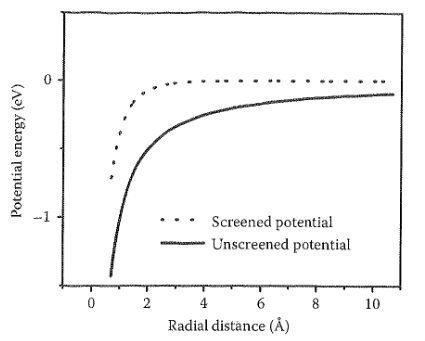
Thus, the potential at \(r\) is Coulomb potential times an exponential factor and is of the form of Yukawa potential. This is called screened Coulomb potential. The potential energy of an electron in the potential of a positive charge is shown schematically in Fig. 10.2. The potential energy for the screened potential approaches zero much faster than for the unscreened potential. The length \(1/k_s\) is a measure of the effective range of the potential and is called the screening distance. In metals, the screening distance is of the order of interatomic spacing but in semiconductors, it is much larger.
10.4 Hohenberg–Kohn Theorems
We saw in the Thomas–Fermi theory that electronic systems could be described in terms of electron density \(n(\vec{r})\). A firm and exact theoretical foundation for such description was provided by Hohenberg and Kohn (1964) who gave two theorems that laid the foundation of the DFT.
The external potential \(v(\vec{r})\) is a unique functional of the electron density \(n(\vec{r})\) (for definition of functional, see Appendix D). As a result, the total ground-state energy \(E\) of any many-electron system is also a unique functional of \(n(\vec{r})\), that is, \(E = E[n]\).
The functional \(E[n]\) for the total energy has a minimum equal to the ground-state energy at the ground-state density.
To prove the first theorem, we assume that there are two different potentials \(v(\vec{r})\) and \(v'(\vec{r})\) with ground states \(\psi\) and \(\psi'\) producing the same density \(n(\vec{r})\). We show that this assumption leads to an absurd result. We assume the ground state to be nondegenerate. The proof also exists for the degenerate case but is more complicated and, therefore, will not be discussed here.
Since \(v'(\vec{r})\neq v(\vec{r})\), \(\psi'\neq\psi\) because these states are the eigenstates of different Hamiltonians. Let us denote the Hamiltonians and ground-state energies associated with \(\psi\) and \(\psi'\) by \(H\), \(H'\) and \(E\), \(E'\), respectively. Then, from Raleigh–Ritz variational principle, we have
\[ E = \langle\psi|H|\psi\rangle < \langle\psi'|H|\psi'\rangle \tag{10.21}\]
Now
\[ \begin{aligned} \langle\psi'|H|\psi'\rangle &= \langle\psi'|H'+(H-H')|\psi'\rangle \\[6pt] &= \langle\psi'|H'|\psi'\rangle + \langle\psi'|V-V'|\psi'\rangle \\[6pt] &= E' + \int\bigl(v(\vec{r})-v'(\vec{r})\bigr)\,n(\vec{r})\,d^3r \end{aligned} \tag{10.22}\]
where we have used Eq. 10.4. Thus, from Eq. 10.21, we get
\[ E < E' + \int\bigl(v(\vec{r})-v'(\vec{r})\bigr)\,n(\vec{r})\,d^3r \tag{10.23}\]
Similarly, by interchanging primed and unprimed quantities, we get
\[ E' < E + \int\bigl(v'(\vec{r})-v(\vec{r})\bigr)\,n(\vec{r})\,d^3r \tag{10.24}\]
by adding Eq. 10.23 and Eq. 10.24, we get
\[ E + E' < E + E' \]
which is absurd.
Thus, we conclude that electron density \(n(\vec{r})\) associated with the ground state corresponding to an external potential \(v(\vec{r})\) cannot be reproduced by the ground-state density corresponding to a different potential \(v'(\vec{r})\) (except when \(v'(\vec{r})-v(\vec{r})=\text{constant}\)). Thus, it follows that the ground-state electron density \(n(\vec{r})\) determines \(v(\vec{r})\) uniquely. This further implies that \(n(\vec{r})\) is produced by unique \(H\). Since \(H\) uniquely determines the nondegenerate ground state of the system, \(n(\vec{r})\) also determines the ground-state wave function uniquely. Hence, \(E = \langle\psi|H|\psi\rangle = E[n(\vec{r})]\) is uniquely determined by \(n(\vec{r})\) only. Note that since \(n(\vec{r})\) determines \(H\) uniquely, therefore, it determines not only the ground state but all the excited states as well. However, here we shall focus on the ground state of the system.
To prove the second theorem, let us write the ground-state energy \(E[n(\vec{r})]\) as
\[ \begin{aligned} E[n(\vec{r})] &= \langle\psi|V|\psi\rangle + \langle\psi|T+V_{EE}|\psi\rangle \\[6pt] &= \int v(\vec{r})\,n(\vec{r})\,d^3r + F[n(\vec{r})] \end{aligned} \tag{10.25}\]
Since \(\psi\) is functional of \(n(\vec{r})\), \(F = \langle\psi|T+V_{EE}|\psi\rangle\) is also functional of \(n(\vec{r})\).
Now, consider a many-electron system with \(N\) electrons in a given external potential \(v(\vec{r})\). This means that we now keep \(v(\vec{r})\) fixed and change \(n(\vec{r})\) (\(n(\vec{r})\) = ground-state electron density). Let us define the following energy functional for the density \(n'(\vec{r})\):
\[ E_v[n'(\vec{r})] = \int v(\vec{r})\,n'(\vec{r})\,d^3r + F[n'(\vec{r})] \tag{10.26}\]
Now, we know that
\[ \tilde{E}_v[\psi'] = \langle\psi'|V|\psi'\rangle + \langle\psi'|T+V_{ee}|\psi'\rangle \]
has lower value for the correct nondegenerate ground-state \(\psi\) than for any other \(\psi'\). Let \(\psi'\) be the state associated with density \(n'(\vec{r})\). Then
\[ \begin{aligned} \tilde{E}_v[\psi'] &= \int v(\vec{r})\,n'(\vec{r})\,d^3r + F[n'(\vec{r})] \\[4pt] &> \tilde{E}_v[\psi] = \int v(\vec{r})\,n(\vec{r})\,d^3r + F[n(\vec{r})] \end{aligned} \tag{10.27}\]
But
\[ \tilde{E}_v[\psi'] = E_v[n'] \]
and
\[ \tilde{E}_v[\psi] = E_v[n] \]
Therefore
\[ E_v[n] < E_v[n'] \]
This proves the second theorem.
The functional \(F[n]\) introduced in Eq. 10.25 is a functional of density \(n(\vec{r})\) and is independent of the external potential \(v(\vec{r})\). It contains kinetic and interaction energies and no exact expression for it is known. However, several good approximations for \(F[n]\) have been developed. Let us first split \(F[n]\) into three parts:
\[ F[n] = T_s[n] + \frac{e^2}{2}\iint\frac{1}{4\pi\varepsilon_0}\frac{n(\vec{r})\,n(\vec{r}')}{|\vec{r}-\vec{r}'|}\,d^3r\,d^3r' + E_{xc}[n] \tag{10.28}\]
where \(T_s[n]\) is the kinetic energy of noninteracting electron gas of density \(n(\vec{r})\) in its ground state, the second term is the classical Coulomb energy, and the remainder \(E_{xc}[n]\) is called exchange–correlation energy. Note that \(E_{xc}[n]\) contains part of the total kinetic energy. The reason why \(T_s[n]\) and not \(\langle T\rangle\) has been separated in Eq. 10.28 will become clear in the following section.
10.5 Derivation of Kohn–Sham (KS) Equations
Using Eq. 10.25 and Eq. 10.28, we can write the total energy functional as
\[ \begin{aligned} E[n] ={}& \int v(\vec{r})\,n(\vec{r})\,d^3r \\[6pt] &+ T_s[n] \\[6pt] &+ \frac{e^2}{2} \iint \frac{1}{4\pi\varepsilon_0} \frac{ n(\vec{r})\,n(\vec{r}') }{ |\vec{r}-\vec{r}'| } \,d^3r\,d^3r' \\[6pt] &+ E_{xc}[n] \end{aligned} \tag{10.29}\]
We have to minimize Eq. 10.29 subject to the condition
\[ \int n(\vec{r})\,d^3r = N \]
This gives
\[ \frac{\delta E[n]}{\delta n(\vec{r})} - \mu = 0 \tag{10.30}\]
or
\[ \frac{\delta T_s[n]}{\delta n(\vec{r})} + v(\vec{r}) + \int\frac{e^2}{4\pi\varepsilon_0}\frac{n(\vec{r}')}{|\vec{r}-\vec{r}'|}\,d^3r' + \frac{\delta E_{xc}[n]}{\delta n(\vec{r})} - \mu = 0 \]
Let us write
\[ v_H(\vec{r}) = \int\frac{e^2}{4\pi\varepsilon_0}\frac{n(\vec{r}')}{|\vec{r}-\vec{r}'|}\,d^3r' \tag{10.31}\]
and
\[ v_{xc}(\vec{r}) = \frac{\delta E_{xc}[n]}{\delta n(\vec{r})} \tag{10.32}\]
where \(v_{xc}(\vec{r})\) incorporates the effects of exchange and correlations and is known as the exchange–correlation potential. Thus, we get
\[ \frac{\delta T_s[n]}{\delta n(\vec{r})} + v(\vec{r}) + v_H(\vec{r}) + v_{xc}(\vec{r}) - \mu = 0 \tag{10.33}\]
where \(\mu\) is the Lagrange multiplier. Eq. 10.33 is the required equation only if it could be solved. Then, it would give us the electron density \(n(\vec{r})\), which in turn would give us the total energy \(E\) from Eq. 10.29. However, there are two problems: (i) functional \(T_s[n]\) is not known and (ii) \(v_{xc}(\vec{r})\) is also unknown. Thus, Eq. 10.33 can be solved only approximately. We first note that Eq. 10.33 reduces to the Thomas–Fermi equation if one neglects \(v_{xc}(\vec{r})\) and uses
\[ T_s[n] = C_k\int n(\vec{r})^{5/3}\,d^3r \]
Better functionals for \(T_s[n]\) have been proposed such as Thomas–Fermi–Weizsäcker functional (Weizsäcker 1935). But such theories had only limited success so far and could not predict the shell structure for atoms.
Another approach to solve Eq. 10.33 is due to Kohn and Sham (1965) who had to introduce orbitals in the DFT. They noted that if the last term in Eq. 10.29, that is, \(E_{xc}[n]\), was absent, then the expression would be identical to Hartree’s expression for energy. Then, \(v_{xc}(\vec{r})\) would be absent in Eq. 10.33 too and this equation could be solved by using
\[ n(\vec{r}) = \sum_{i=1}^{N}|\psi_i(\vec{r})|^2 \tag{10.34}\]
and by solving
\[ \left(-\frac{\hbar^2}{2m_e}\nabla^2 + v(\vec{r}) + v_H(\vec{r})\right)\psi_i(\vec{r}) = \varepsilon_i\psi_i(\vec{r}) \tag{10.35}\]
Thus, if one could write \(n(\vec{r})\) in terms of single-particle orbitals as in Eq. 10.34 even when \(v_{xc}(\vec{r})\) is present, Eq. 10.33 could be solved in a similar way. Thus, we define
\[ v_{eff}(\vec{r}) = v(\vec{r}) + v_H(\vec{r}) + v_{xc}(\vec{r}) \tag{10.36}\]
and use
\[ n(\vec{r}) = \sum_{i=1}^{N}|\psi_i(\vec{r})|^2 \tag{10.37}\]
Then, in analogy with Eq. 10.35, \(\psi_i(\vec{r})\) can be obtained by solving
\[ \left[-\frac{\hbar^2}{2m_e}\nabla^2 + v_{eff}(\vec{r})\right]\psi_i(\vec{r}) = \varepsilon_i\psi_i(\vec{r}) \tag{10.38}\]
Eq. 10.38 is known as KS equations and \(\psi_i(\vec{r})\), \(\varepsilon_i\), and \(v_{eff}(\vec{r})\) as KS orbitals, KS energies, and KS potential, respectively. The Hamiltonian
\[ H = -\frac{\hbar^2}{2m_e}\nabla^2 + v_{eff}(\vec{r}) \]
is called as the KS Hamiltonian.
The KS equations have to be solved self-consistently. Note that the orbitals in the DFT are introduced via Eq. 10.37, that is, we are assuming that \(n(\vec{r})\) can always be expressed in terms of orbitals by Eq. 10.37. In other words, we are mapping our interacting electron system onto an auxiliary system of independent particles, which has the same density as our original system. These independent particles move in a potential given by Eq. 10.36. This (Eq. 10.37) is an ansatz that enabled Kohn and Sham to arrive at Eq. 10.38 and hence it provided a way to solve the many-electron problem. Note the simplicity of Eq. 10.38, which reduces the many-electron problem to a one-electron problem. This is similar to Hartree or H–F methods but unlike these methods, this includes the effects of exchange and correlations. Note that the exchange–correlation potential \(v_{xc}(\vec{r})\) is an unknown function for which some approximation has to be made if we want to solve the problem. This will be done in the next section.
Let us now express the total energy in terms of \(\varepsilon_i\). To do this, multiply Eq. 10.38 by \(\psi_i^*(\vec{r})\) from the left and integrate over \(\vec{r}\). This gives
\[ \varepsilon_i = \int\psi_i^*(\vec{r})\left[-\frac{\hbar^2}{2m_e}\nabla^2 + v_{eff}(\vec{r})\right]\psi_i(\vec{r})\,d^3r \]
or
\[ \begin{aligned} \sum_i\varepsilon_i &= \sum_i\int\psi_i^*(\vec{r})\left[-\frac{\hbar^2}{2m_e}\nabla^2\right]\psi_i(\vec{r})\,d^3r \\[6pt] &\quad + \sum_i\int\psi_i^*(\vec{r})\,\psi(\vec{r})\,v(\vec{r})\,d^3r + \sum_i e^2\int\frac{1}{4\pi\varepsilon_0}\frac{\psi_i^*\psi_i\,n(\vec{r}')}{|\vec{r}-\vec{r}'|}\,d^3r\,d^3r' \\[6pt] &\quad + \sum_i\int v_{xc}(\vec{r})\,\psi_i^*(\vec{r})\,\psi_i(\vec{r})\,d^3r \\[6pt] &= T_s[n] + \int v(\vec{r})\,n(\vec{r})\,d^3r + e^2\iint\frac{1}{4\pi\varepsilon_0}\frac{n(\vec{r})\,n(\vec{r}')}{|\vec{r}-\vec{r}'|}\,d^3r\,d^3r' \\[6pt] &\quad + \int v_{xc}(\vec{r})\,n(\vec{r})\,d^3r \end{aligned} \tag{10.39}\]
By comparing Eq. 10.29 and Eq. 10.39, we can write
\[ \begin{aligned} E ={}& \sum_i \varepsilon_i \\[6pt] &- \frac{e^2}{2} \iint \frac{1}{4\pi\varepsilon_0} \frac{ n(\vec{r})\,n(\vec{r}') }{ |\vec{r}-\vec{r}'| } \,d^3r\,d^3r' \\[6pt] &+ E_{xc}[n] \\[6pt] &- \int v_{xc}(\vec{r})\,n(\vec{r})\,d^3r \end{aligned} \tag{10.40}\]
Note that in the KS theory, \(T_s[n]\) is treated exactly.
10.6 Local Density Approximation (LDA)
The exact form of \(F[n]\) or \(E_{xc}[n]\) (or \(v_{xc}(\vec{r})\)) is not known, but approximations have been developed to calculate these quantities. The first such approximation was developed by Kohn and Sham (1965) and is known as the LDA, which has been highly successful in calculating the electronic structure of atoms, molecules, and solids. It is assumed that the electron density \(n(\vec{r})\) varies very slowly in space, so that the electron gas in a small-volume element \(d^3r\) could be considered locally uniform. Therefore, one could use the exchange–correlation energy of the homogeneous electron gas to evaluate \(E_{xc}[n]\) as follows. If \(\varepsilon_{xc}(n)\) is the exchange–correlation energy per particle of a uniform electron gas of density \(n\), the exchange–correlation energy of the uniform gas of density \(n(\vec{r})\) in volume \(d^3r\) is \(\varepsilon_{xc}(n(\vec{r}))\,n(\vec{r})\,d^3r\). Therefore, the exchange–correlation energy of the system with slowly varying density can be written as
\[ E_{xc}[n] = \int\varepsilon_{xc}\!\bigl(n(\vec{r})\bigr)\,n(\vec{r})\,d^3r \tag{10.41}\]
This is known as the LDA.
In the LDA, \(v_{xc}(\vec{r})\) can be found by using Eq. 10.32 and Eq. 10.41 as
\[ \begin{aligned} v_{xc}(\vec{r}) &= \frac{\delta E_{xc}[n]}{\delta n(\vec{r})} = \frac{d}{dn}\Bigl(\varepsilon_{xc}\!\bigl(n(\vec{r})\bigr)\,n(\vec{r})\Bigr) \\[6pt] &= \mu_{xc}\!\bigl(n(\vec{r})\bigr) \end{aligned} \tag{10.42}\]
where \(\mu_{xc}(n)\) is the exchange and correlation contributions to the chemical potential of the uniform electron gas.
Using Eq. 10.40 through Eq. 10.42, the total energy can be written in the LDA as
\[ \begin{aligned} E ={}& \sum_i \varepsilon_i \\[6pt] &- \frac{e^2}{2} \iint \frac{1}{4\pi\varepsilon_0} \frac{ n(\vec{r})\,n(\vec{r}') }{ |\vec{r}-\vec{r}'| } \,d^3r\,d^3r' \\[6pt] &+ \int \Bigl( \varepsilon_{xc}\!\bigl(n(\vec{r})\bigr) - \mu_{xc}\!\bigl(n(\vec{r})\bigr) \Bigr) n(\vec{r}) \,d^3r \end{aligned} \tag{10.43}\] As mentioned in Chapter 2, the homogeneous electron gas has been studied by various workers. Several analytic fits to theoretically calculated \(\varepsilon_{xc}(n)\) have been proposed. The one proposed by Gunnarsson and Lundqvist (1976) in atomic units (see Appendix C) is
\[ \varepsilon_{xc}(n) = -\frac{0.458}{r_s} - 0.0666\;G\!\left(\frac{r_s}{11.4}\right) \tag{10.44}\]
where \(G(x)\) is defined as
\[ G(x) = \frac{1}{2}\left[(1+x^3)\ln(1+x^{-1}) - x^2 + x/2 - 1/3\right] \]
The correlation energy of the homogeneous electron gas has also been calculated by using the quantum Monte Carlo method by Ceperley and Alder (1980), which is considered to be a very accurate calculation. This has been fitted to analytical forms by Perdew and Zunger (1981) and Vosko et al. (1980). These fitted forms are used in most of the current electronic structure calculations.
As can be seen from the above discussion, the LDA should be a good approximation if the electron density \(n(\vec{r})\) is slowly varying. However, it has yielded surprisingly good results even in cases where the density is not slowly varying. For metals, the theory does extremely well. In semiconductors, the band gap is underestimated by a 1/2–2/3 factor. Insulators, particularly Mott insulators, are not described well. Intense efforts are going on to remedy these defects of the theory. We shall briefly discuss these effects later.
10.7 Comparison of the DFT with the Hartree and H–F Theories
To make the comparison, let us split the exchange–correlation energy \(E_{xc}[n]\) in Eq. 10.41 into exchange and correlations parts, that is
\[ \begin{aligned} E ={}& \int v(\vec{r})\,n(\vec{r})\,d^3r \\[6pt] &+ T_s[n] \\[6pt] &+ \frac{e^2}{2} \iint \frac{1}{4\pi\varepsilon_0} \frac{ n(\vec{r})\,n(\vec{r}') }{ |\vec{r}-\vec{r}'| } \,d^3r\,d^3r' \\[6pt] &+ E_x[n] \\[6pt] &+ E_c[n] \end{aligned} \tag{10.45}\] The exact equations of Hartree theory are obtained from Eq. 10.45 by dropping \(E_x + E_c\). The H–F equations are obtained by dropping \(E_c\). Obviously, the inclusion of any reasonable approximation will improve these equations, which is done in the LDA. The advantage of using the KS equations in the LDA is that these equations are as simple as the Hartree equations but in most cases they give very good account of exchange and correlation effects. In practice, it is found that for solids the KS results are better than H–F results, although the latter are much more computationally demanding. The reason is that the KS equation includes fairly accurately, both exchange and correlations, while the H–F equation includes exchange only but neglects correlations completely.
10.8 Comments on the KS Eigenvalues and KS Orbitals
Although the DFT provides a scheme to reduce the entire many-body problem to a Schrödinger-like single-particle equation, the physical meaning of \(\varepsilon_i\) is not clear. Often, these eigenvalues have been used to interpret excitation spectra and in most cases good agreement with experimental results was found. But there are problematic cases too.
There is a special case when \(\varepsilon_i\) does have a physical meaning. For infinite systems, the highest occupied level \(\varepsilon_N\) equals the chemical potential, that is, \(\varepsilon_N = \mu\), provided highest occupied orbitals are extended. This is a density functional analog of Koopmans’ theorem, which we shall now prove.
Let us consider an infinite system in which eigenfunction \(\psi_i\) at the maximum occupied single-particle energy \(\varepsilon_F\) is all extended. We shall calculate the difference in ground-state energies of \(N\) and \((N+m)\) particles for \(m \ll N\).
Change in \(n(\vec{r})\) as a result of adding \(m\) particle is
\[ \delta n(\vec{r}) = \sum_{i=N+1}^{N+m}|\psi_i(\vec{r})|^2 \tag{10.46}\]
Also, the change in ground-state energy
\[ \begin{aligned} \delta E[n] &= T_s\bigl[n(\vec{r})+\delta n(\vec{r})\bigr] - T_s\bigl[n(\vec{r})\bigr] \\[6pt] &\quad + \int\delta n(\vec{r})\left[v(\vec{r}) + \int\frac{e^2}{4\pi\varepsilon_0}\frac{n(\vec{r}')}{|\vec{r}-\vec{r}'|}\,d^3r' + \frac{\delta E_{xc}}{\delta n(\vec{r})}\right]d^3r \\[6pt] &= \sum_{i=N+1}^{N+m}\int -\frac{\hbar^2}{2m_e}\psi_i^*(\vec{r})\nabla^2\psi_i(\vec{r})\,d^3r \\[6pt] &\quad + \sum_{i=N+1}^{N+m}|\psi_i(\vec{r}')|^2\left[v(\vec{r}) + \int\frac{e^2}{4\pi\varepsilon_0}\frac{n(\vec{r}')}{|\vec{r}-\vec{r}'|}\,d^3r' + \frac{\delta E_{xc}}{\delta n(\vec{r}')}\right]d^3r \\[6pt] &= \sum_{i=N+1}^{N+m}\varepsilon_i = m\varepsilon_F \end{aligned} \tag{10.47}\]
Now
\[ \int\delta n(\vec{r})\,d^3r = m \]
\[ \therefore\quad \delta E\bigl[n(\vec{r})\bigr] = \varepsilon_F\int\delta n(\vec{r})\,d^3r \]
or
\[ \frac{\delta E[n]}{\delta n(\vec{r})} = \varepsilon_F \]
But from Eq. 10.30
\[ \frac{\delta E[n]}{\delta n(\vec{r})} = \mu \]
\[ \therefore\quad \varepsilon_F = \mu \tag{10.48}\]
This proves the theorem.
Similarly, one should remember that KS orbital \(\psi_i(\vec{r})\) enters in the DFT via Eq. 10.37, through its relation with electron charge density. Thus, there is no reason to regard the Slater determinant constructed from \(\psi_i\)’s as the true many-electron wave function, that is, \(\psi_i(\vec{r})\) is not the one-electron wave function in the sense of the H–F approximation.
10.9 Extensions to Magnetic Systems
So far, we have only discussed nonmagnetic systems at absolute zero temperature. The DFT has been generalized to the ground state of magnetic systems by von Barth and Hedin (1972), Pant and Rajagopal (1972), and Rajagopal and Callaway (1973) and to finite temperatures by Mermin (1965). Here, we shall briefly discuss the extension to magnetic systems. This extension of the theory to magnetic systems is known as spin DFT. For simplicity, we assume that the system is in a magnetic field \(B(\vec{r})\), which is pointing in only one direction that we assume our \(z\) direction. Also, we assume that the electronic spin is either up (\(\sigma = +1\) along the magnetic field) or down (\(\sigma = -1\)). Thus, the total density \(n(\vec{r})\) is equal to the sum of two densities \(n_\uparrow(\vec{r})\) and \(n_\downarrow(\vec{r})\)
\[ n(\vec{r}) = n_\uparrow(\vec{r}) + n_\downarrow(\vec{r}) = \sum_\sigma n_\sigma(\vec{r}) \]
The exchange–correlation function is now functional of \(n_\uparrow(\vec{r})\) and \(n_\downarrow(\vec{r})\)
\[ E_{xc} = E_{xc}[n_\uparrow,\,n_\downarrow] \]
Following similar arguments as discussed earlier, we obtain the KS equation as
\[ \left[-\frac{\hbar^2}{2m_e}\nabla^2 + v_{eff}^\sigma(\vec{r})\right]\psi_{i\sigma}(\vec{r}) = \varepsilon_{i\sigma}\,\psi_{i\sigma}(\vec{r}) \quad [\sigma = \pm 1] \tag{10.49}\]
where
\[ \begin{aligned} v_{eff}^\sigma(\vec{r}) &= v(\vec{r}) - \sigma\mu_B B(\vec{r}) + \frac{e^2}{4\pi\varepsilon_0}\int\frac{n(\vec{r}')}{|\vec{r}-\vec{r}'|}\,d^3r' + \frac{\delta E_{xc}[n_\uparrow,n_\downarrow]}{\delta n_\sigma(\vec{r})} \quad [\sigma = \pm 1] \end{aligned} \tag{10.50}\]
and
\[ n_\sigma(\vec{r}) = \sum_{\text{occupied}}|\psi_{i\sigma}|^2 \tag{10.51}\]
\(\mu_B = e\hbar/2m_e\) is the Bohr magneton and \(\varepsilon_{i\sigma}\) are the Lagrange multipliers. As was the case for nonmagnetic systems, the exact form of the exchange–correlation functional \(E_{xc}[n_\uparrow, n_\downarrow]\) is not known and approximations have been developed for it. Similar to the LDA, one can make local approximation, known as local spin density approximation (LSDA). For more details, we refer to the book by Parr and Yang (1989).
10.10 Performance of the LDA/LSDA
The LDA and LSDA have proved to be remarkably good approximations. Considering that these approximations were derived by assuming slowly varying densities, they give very good results for atoms, molecules, and solids. Some of the successes of LDA/LSDA are
- Ground-state geometries are given accurately.
- Charge densities are better than 2%.
- Most of the time, LDA results are better than H–F results.
- Physical trends are given correctly (e.g., see Moruzzi et al. 1978).
- Equilibrium distances are given reasonably well typically with an accuracy of 1% although somewhat underestimated.
However, LDA/LSDA fails in many cases. Some of their failures are
- LDA underestimates band gaps in semiconductors. For example, LDA gives a band gap of Si about 0.5 eV compared to the experimental result of about 1.1 eV.
- FeO and CoO, which are insulators, are predicted to be metallic.
- Fe is predicted to be an fcc paramagnet rather than bcc ferromagnet at low temperatures.
- LDA predicts incorrect ground state for many atoms.
- LDA predicts unstable negative atomic ions.
- It may fail in weak molecular bonds, for example, in hydrogen bonds as in the bonding region the charge density is very small. It may fail in van der Waal’s systems too.
- LDA overbinds molecules and solids.
10.11 Beyond LDA
We saw that in most cases, the LDA/LSDA is adequate. However, in cases where higher accuracy is desired, one must go beyond the LDA. For example, an error of 1 eV in binding energy is not acceptable in the study of chemical reactions. Similarly, higher accuracy is needed in the study of phase transformations or if one wants to use the theory for materials design. What one would like is the accuracy of 0.1 eV or less in the calculation of binding energy. Several attempts have been made in this direction although success has been rather limited. We shall summarize few such attempts in this direction.
10.11.1 Generalized Gradient Approximations (GGAs)
We had seen that the LDA/LSDA was derived by assuming that the electron density varies very slowly in space. Thus, it was argued that LDA/LSDA could be improved if we expanded the exchange–correlation functional in terms of gradient of the density in Taylor series and truncated it at some order. Such an approximation is known as gradient expansion approximation (GEA) and was implemented by Herman et al. (1969). It turned out that such an approximation often gave worse results and did not provide any improvement over LDA. The reason for this seems to be that gradients of the density in real system become very large; as a result, such an expansion breaks down. Also, it was found that the GEA does not satisfy certain sum rules. Later on, it was realized that there was no need of such an expansion and it was possible to construct exchange–correlation functional, which was a functional of density as well as its gradient and satisfied the sum rules. This could be written as
\[ E_{xc}^{GGA}[n_\uparrow,n_\downarrow] = \int d^3r\;f\!\bigl(n_\uparrow(\vec{r}),\,n_\downarrow(\vec{r}),\,\nabla n_\uparrow,\,\nabla n_\downarrow\bigr) \tag{10.52}\]
In contrast to LSDA, there are many functions \(f\) that are in use. One that has been widely used is by Perdew and Wang, known as PW91 (Perdew 1991). Later on, Perdew et al. (1996) proposed another functional (PBE), which retains important features of PW91.
The GGA often provides results for structural and magnetic properties of materials that are better than LDA results and are closer to experimental values. For example, the GGA gives lattice constants that are closer to experimental values and also gives the correct ground state for ferromagnetic Fe. However, it also fails sometimes. At times it overcorrects LDA bond lengths and gives values that are up to 2% larger than experimental values. Also, sometimes cohesive energy is 10–20% too small. The GGA gives poor results for ferroelectrics, and also like LDA it does not give correct band gaps for semiconductors. It does not give good results for strongly correlated systems and present research is still continuing in search of a better functional.
10.11.2 LDA + U Method
We had seen that LSDA and GGA fail to give the correct ground state of strongly correlated systems such as transition metal oxides. LDA + U or GGA + U methods have been designed to correct this situation by constructing an orbital-dependent functional. The idea has been taken from the Hubbard model (Hubbard 1963). Suppose we have an orbital that already has one electron. If we put another electron in it, it will cost an energy U because of the electron–electron repulsion in that orbital. This idea when incorporated in LSDA or GGA produces LDA + U method.
To implement the above idea, the electrons are subdivided into two subsystems; \(d\) or \(f\) electrons, which interact strongly with Coulomb repulsion U and \(s\), and \(p\) electrons, which are well described by the LDA or GGA. For \(d\) (or \(f\)) electrons, an extra term is added to the LDA functional equal to \((1/2)\,\mathrm{U}\sum_{i,j,\,i\neq j}n_i\,n_j\), where \(n_i\), \(n_j\) are \(d\) occupancies. Thus, the LDA + U functional can be written as
\[ E_{\mathrm{LDA+U}} = E_{\mathrm{LDA}} - \frac{U}{2}N_d(N_d-1) + \frac{1}{2}\,\mathrm{U}\sum_{\substack{i,j \\ i\neq j}}n_i\,n_j \tag{10.53}\]
where \(N_d = \sum_i n_i\) is total number of \(d\) electrons.
This orbital-dependent functional gives upper and lower Hubbard band separation equal to U and thus correctly describes the physics of Mott insulators. For details of the method, we refer to the review article by Animosov et al. (1997). This approach has been further extended to include dynamical correlations within dynamical mean-field theory (DMFT) and known as LDA + DMFT (see, e.g., Savrasov et al. 2000).
The LDA + U method has proved quite successful in reproducing the correct ground state of strongly correlated systems. For example, it correctly gives the antiferromagnetic insulating ground states for many transition metal oxides and cuprate superconductors, which turn out to be metallic using LSDA or GGA. The main problem of the LDA + U method is the choice of the value of U. Although U can be found ab initio by using the constrained DFT approach, it is overestimated by this method. Thus, the common way of finding U is to treat it as an adjustable parameter so that one finds good agreement between some calculated and experimental results.
10.11.3 Self-Interaction Correction (SIC) Method
In any theory, there should be no self-interaction as an electron cannot interact with itself. Recall that in H–F approximations, the Coulomb interaction energy of an electron in a given state with itself is exactly canceled by its exchange interaction. Thus, there was no problem in H–F theory as far as the self-interaction was concerned. However, in the LDA, the self-interaction is not canceled properly and, therefore, a self-interaction correction is required.
Perdew and Zunger (1981) proposed a self-interaction corrected exchange–correlation energy functional, which is also an orbital-dependent functional. Results for atoms show that SIC corrects most of the errors of the LDA. Also, using SIC, stable solutions for negative ions can be obtained. Thus, SIC leads to highly accurate results for atomic systems. However, the method is easily applicable to systems where electronic orbitals are localized, but for extended orbitals, it is very difficult to apply. Calculations for band gaps of insulators show a marked improvement over the LDA results.
10.11.4 GW Method
We saw that neither the LDA nor the GGA gave correct band gaps for semiconductors. This is because the calculation of band gap involves an excited state and the LDA and GGA do not give it correctly because both of them are ground-state theories. Thus, to get the band gap correctly, we have to develop a theory that can give excited states correctly and this is what the GW method does. It has been shown that single-particle energies can be obtained by solving the equation
\[ \begin{aligned} \left( -\frac{\hbar^2}{2m_e}\nabla^2 + v(\vec{r}) + v_H(\vec{r}) \right)\psi_i(\vec{r}) & \\ + \int d^3r'\; \Sigma(\vec{r},\vec{r}',\varepsilon)\, \psi_i(\vec{r}') &= \varepsilon_i\,\psi_i(\vec{r}) \end{aligned} \tag{10.54}\]
where \(v_H(\vec{r})\) is the Hartree potential and \(\Sigma\) is called self-energy, which includes the effects of exchange and correlations. A comparison with H–F equation shows that in the H–F theory, this corresponds to the exchange interaction. Thus, in any theory better than H–F, this term should contain exchange as well as correlation effects. The problem is that \(\Sigma\) is unknown and has to be approximated. In the GW method, \(\Sigma\) is approximated by a product involving the Green’s function \(G\) and screened Coulomb interaction \(W\), which can be written symbolically as
\[ \Sigma = iGW \tag{10.55}\]
This factorization gives the “GW” name to the method. Note that if instead of \(W\) the bare Coulomb interaction is taken, one obtains the H–F method that gives pathological results for the density of states for the free electron gas. We see that this behavior was linked to the long-range tail of the bare Coulomb interaction. Since in the GW method, screened Coulomb interaction is used, such a situation does not arise. Formulation of the GW method is quite complicated and for details we refer to the review article by Aryasetiawan and Gunnarsson (1998).
One of the great successes of the GW method is that it gives the band gaps of semiconductors in good agreement with experiments. However, the method is difficult to implement and is computationally very expensive. Another method that has been developed by Harbola and collaborators based on splitting the \(k\)-space also gives correct band gaps for a large number of semiconductors but is much simpler than the GW method (Samal and Harbola 2006, Rahaman et al. 2009). A recently developed functional TB-mBJ also gives a band gap of semiconductors and insulators in agreement with experiments (Tran and Blaha 2009).
10.12 Time-Dependent Density Functional Theory (TDDFT)
The DFT has been generalized to include time-dependent potentials and is known as TDDFT. This theory can be thought of as a reformulation of the time-dependent quantum mechanics in terms of time-dependent electron density \(n(\vec{r},t)\). This approach has a great advantage over the wave function approach, as the many-body wave function is a function of \(N\) positions, where \(N\) is the number of electrons while the electron density is a function of one position only.
The TDDFT was developed due to the pioneering work of Runge and Gross (1984) who gave a theorem known as Runge–Gross theorem, which is the analog of the Hohenberg–Kohn theorem for the time-dependent electron density \(n(\vec{r},t)\). The theorem establishes a one-to-one correspondence between \(n(\vec{r},t)\) and time-dependent external potential \(v_{ext}(\vec{r},t)\) for a given initial state. Unlike in DFT, there is no energy minimum principle in the TDDFT. Instead, the formulation of TDDFT is based on the stationary action principle. Similar to DFT, one can define a fictitious system of noninteracting electrons that has the same density \(n(\vec{r},t)\) of the real system and which moves in a time-dependent effective potential \(v_{eff}(\vec{r},t)\). This leads to an equation similar to the time-dependent Schrödinger equation, known as the time-dependent KS equation:
\[ i\hbar\frac{\partial}{\partial t}\psi_i(\vec{r},t) = \left[-\frac{\hbar^2}{2m_e}\nabla^2 + v_{eff}(\vec{r},t)\right]\psi_i(\vec{r},t) \tag{10.56}\]
where
\[ \begin{aligned} v_{eff}(\vec{r},t) &= v_{ext}(\vec{r},t) + v_{xc}(\vec{r},t) \\ &\quad + e^2\int\frac{1}{4\pi\varepsilon_0} \frac{n(\vec{r}',t)}{|\vec{r}-\vec{r}'|}\,d^3r' \end{aligned} \tag{10.57}\]
Here, \(v_{xc}(\vec{r},t)\) is the time-dependent exchange–correlation potential and \(n(\vec{r},t)\) is given by
\[ n(\vec{r},t) = \sum_i|\psi_i(\vec{r},t)|^2 \tag{10.58}\]
The exchange–correlation potential \(v_{xc}(\vec{r},t)\) is an unknown functional of \(n(\vec{r},t)\), which has to be approximated. The simplest approximation is the adiabatic local density approximation (ALDA) in which exchange–correlation potential of the uniform gas with the instantaneous density is used to evaluate \(v_{xc}(\vec{r},t)\), that is
\[ v_{xc}^{\mathrm{ALDA}}(\vec{r},t) = v_{xc}^{\mathrm{unif}}\!\bigl(n(\vec{r},t)\bigr) \tag{10.59}\]
This formalism has been applied to calculate excited-state energies and photo-absorption cross sections of molecules and clusters. The excited-state energies of the system can be found by calculating the linear response function, which has poles at the excitation energies. This field is still developing and has several challenges ahead, for example, developing theory beyond ALDA, and so on. For further details, we refer to the book by Gross and Dreizler (1995).
10.13 Exercises
(a) Dirac extended the Thomas–Fermi method by including the approximate form of the exchange energy given by
\[ -\frac{3}{4}\!\left(\frac{3}{\pi}\right)^{1/3}\int n(\vec{r})^{4/3}\,d^3r \]
Using the variational principle, derive the equation satisfied by \(n(\vec{r})\).
(b) The above model was further extended by Weizsäcker who proposed the correction to the kinetic energy functional given by
\[ \frac{1}{8}\int\frac{|\nabla n(\vec{r})|^2}{n(\vec{r})}\,d^3r \]
Using the variational principle, derive the equation satisfied by \(n(\vec{r})\) (see Parr and Yang (1989) for taking the functional derivative of the above term).
Suppose we have two types of particles with densities \(n_1(\vec{r})\) and \(n_2(\vec{r})\) with internal energy \(U[n_1,n_2]\) such that the total energy \(E\) can be written as
\[ E[n_1,n_2] = U[n_1,n_2] + \int v_{ext}(\vec{r})\,n(\vec{r})\,d^3r \]
where \(n = n_1(\vec{r}) + n_2(\vec{r})\). Show that the total energy is a functional of only \(n\).
(a) Write the Kohn–Sham equation for the electron in a hydrogen atom.
(b) Estimate the LDA exchange energy for the hydrogen atom and compare it with the exact result.
(c) Estimate the LDA total energy of the hydrogen atom and compare it with the exact energy.
Write the Kohn–Sham equation for an electron in the jellium model. What are the Kohn–Sham orbitals and energies? Plot the energy eigenvalues taking parameters corresponding to Na and compare your result with the Hartree and H–F results.
Show that the self-interaction term is exactly canceled in the H–F approximation.
10.14 Further Reading
Dreizler R. M. and Gross E. K. U. 1990. Density Functional Theory: An Approach to the Quantum Many-Body Problem. Berlin: Springer.
Kohn W. 1999. Nobel lecture: Electronic structure of matter wave functions and density functionals. Rev. Mod. Phys. 71:1253–1266.
Lundqvist S. and March N. H. Eds. 1983. Theory of the Inhomogeneous Electron Gas. New York: Plenum Press.
Martin R. M. 2004. Electronic Structure, Basic Theory and Practical Methods. Cambridge: Cambridge University Press.
Parr R. G. and Yang W. 1989. Density Functional Theory of Atoms and Molecules. New York: Oxford University Press.