16 First-Principles Molecular Dynamics
16.1 Introduction
Until now we had assumed that the ions were fixed at their ionic positions and focused on the electronic structure problem, that is we know how to calculate electronic band structure and the total electronic energy using the first-principles approach for a fixed ionic configuration. Now, we will relax the condition that the ions are fixed. We shall see that it is possible to study ion dynamics from the first principles, which, in the most general form, is known as the first-principles molecular dynamics (MD).
MD is a computer simulation technique in which one looks at the time evolution of a system of interacting particles by integrating their equations of motion. In this way, one obtains trajectory of each particle, that is, their coordinates as a function of time. Thus, the technique allows one to view each particle as it moves; therefore, it is like a “theoretical microscope” by which one can see very fine details of a process occurring in a system as a function of time. The technique is also called “computer experiment.” The physical properties are obtained by taking their time averages over the trajectories. Thus, MD is basically a statistical mechanics method.
MD can be of two types (i) classical MD and (ii) first-principles MD. In the classical MD, one uses empirical potentials, while in the first-principles MD the potential is obtained quantum mechanically without using any empirical parameter. Classical MD, although first introduced by Alder and Wainwright (1959) for hard spheres, was developed by Rahman (1964) using empirical potentials. The first-principles MD was first proposed by Bendt and Zunger (1983) and is known as Born-Oppenheimer MD. However, they were not able to implement it on real systems. Car and Parrinello (1985) proposed another way of first-principles MD, which is known as Car-Parrinello MD and also implemented it on a real system (crystalline silicon) to calculate its static and dynamical properties. The development of Car-Parrinello MD has been a major development in the field of electronic structure.
The chapter is organized as follows. In Section Section 16.2, we will discuss the classical MD and in Section Section 16.3, we show how one can calculate physical properties. In Section Section 16.4, we derive basic equations leading to the Born-Oppenheimer MD. In Section Section 16.5, Car-Parrinello MD is discussed. In Section Section 16.6, we give a brief discussion on comparison of the Born-Oppenheimer and Car-Parrinello MD. In Sections Section 16.7 and Section 16.8, we discuss the method of steepest descent (SD) and simulated annealing to obtain the ground state. In Section Section 16.9, we discuss the Hellmann-Feynman theorem and in Section Section 16.10 the calculation of forces. In Section Section 16.11, we mention some applications of the first-principles MD.
16.2 Classical MD
Suppose we have \(N\) atoms in a fixed volume \(\Omega\) interacting via some interparticle potential \(V(\vec R_1,\vec R_2,\ldots,\vec R_N)\), where \(\vec R_i\) are atomic coordinates. We denote velocities by \(\dot{\vec R}_i\), accelerations by \(\ddot{\vec R}_i\), and assume that the atoms are classical particles and follow Newton’s laws. Force \(\vec F_i\) on \(i\)th atom is given by
\[ \vec F_i=-\vec\nabla_i V \tag{16.1}\]
Once the force \(\vec F_i\) is known, one can write Newton’s equation of motion
\[ M\ddot{\vec R}_i=-\vec\nabla_i V \tag{16.2}\]
where we have assumed that each atom has the same mass. In MD, one solves the equations of motion (Eq. 16.2) numerically and studies the time evolution of the system. In classical MD, \(V\) is a phenomenological potential, which is generally obtained by assuming a parametric form and then fitting it to some experimental results. For example, for inert gases, it could be expressed as a sum over Lennard-Jones potentials (see, e.g., Rahman 1964).
The equations of motion (Eq. 16.2) can be integrated numerically by using, for example, Verlet algorithm (Verlet 1967). By using Taylor expansion, one can write
\[ \vec R_i(t+\Delta t)=\vec R_i(t)+\Delta t\dot{\vec R}_i(t)+\frac{(\Delta t)^2}{2}\ddot{\vec R}_i(t)+\frac{(\Delta t)^3}{6}\dddot{\vec R}_i(t)+O[\Delta t^4] \tag{16.3}\]
where \(\Delta t\) is a small interval of time of the order of \(10^{-14}\) s. Similarly,
\[ \vec R_i(t-\Delta t)=\vec R_i(t)-\Delta t\dot{\vec R}_i(t)+\frac{(\Delta t)^2}{2}\ddot{\vec R}_i(t)-\frac{(\Delta t)^3}{6}\dddot{\vec R}_i(t)+O[\Delta t^4] \tag{16.4}\]
Adding Equations Eq. 16.3 and Eq. 16.4, we get
\[ \vec R_i(t+\Delta t)=2\vec R_i(t)-\vec R_i(t-\Delta t)+(\Delta t)^2\ddot{\vec R}_i(t)+O[\Delta t^4] \tag{16.5}\]
In Equation Eq. 16.5, one can substitute for \(\ddot{\vec R}_i(t)\) from Equation Eq. 16.2. Thus, if one knows \(\vec R_i(t)\) and \(\vec R_i(t-\Delta t)\), one can find the positions of atoms at subsequent time intervals. Equation Eq. 16.5 is known as the Verlet algorithm. Note that in the Verlet algorithm the local truncation error varies as \(O[\Delta t^4]\) and therefore, the global error, the total error over the time of interest is of the order of \(\Delta t^2\). Thus, the Verlet algorithm is more efficient than the algorithm based on Equation Eq. 16.3 in which one stops at second derivative of positions. However, it is not a self-starting algorithm, that is, to calculate \(\vec R_i(t+\Delta t)\) one has to know both \(\vec R_i(t)\) and \(\vec R_i(t-\Delta t)\). Therefore, to start it one needs another algorithm such as Equation Eq. 16.3 to obtain first few steps.
Since our system that has a fixed number of particles, \(N\) and volume \(\Omega\), is isolated, the total energy is a constant of motion, that is
\[ E=\frac{1}{2}\sum_i M\dot{\vec R}_i^2+V=\text{constant} \tag{16.6}\]
Here, the velocities at time \(t\) are obtained from
\[ \dot{\vec R}_i(t)=\frac{\vec R_i(t+\Delta t)-\vec R_i(t-\Delta t)}{2\Delta t} \tag{16.7}\]
The time step \(\Delta t\) should be so chosen that the constant of motion (total energy) comes out to be a constant within the desired accuracy.
Using Equations Eq. 16.5 and Eq. 16.7, the phase space trajectories \(\{\vec R_i(t),\dot{\vec R}_i(t)\}\) can be calculated for each atom for several thousand time steps. From this, time average of a physical quantity can be calculated as
\[ \langle A\rangle=\lim_{T\to\infty}\frac{1}{T}\int_{t_0}^{t_0+T}A(t)dt \tag{16.8}\]
Note that at equilibrium, the average cannot depend on initial time \(t_0\). According to the ergodic hypothesis, the time average (Eq. 16.8) provided by MD is the same as the ensemble average. Thus, using Equation Eq. 16.8, one can calculate the temperature of the system as
\[ \frac{3}{2}k_BT=\left\langle\frac{1}{2}\sum_{i=1}^{N}M\dot{\vec R}_i^2\right\rangle =\lim_{T\to\infty}\frac{1}{T}\int_{t_0}^{t_0+T}\frac{1}{2}\sum_{i=1}^{N}M\dot{\vec R}_i^2(t)dt \tag{16.9}\]
where we have assumed that each atom has only 3 degrees of freedom.
It is sometimes useful to define “instantaneous” temperature as
\[ T(t)=\frac{1}{3k_BN}\sum_{i=1}^{N}M\dot{\vec R}_i^2(t) \tag{16.10}\]
Note that this is not a physical quantity as it is not a time-averaged quantity over the trajectories. But it could be used as a helpful device in doing simulations. For more details of classical MD, we refer to the books by Haile (1997), Rapaport (2004), and Allen and Tildesley (1989).
16.3 Calculation of Physical Properties
Once the phase space trajectories have been obtained, physical properties of a system of particles can be calculated by taking the time average over all the trajectories. Here, we shall discuss mean-squared displacement, diffusion constant, velocity auto-correlation function and phonon density of states. The formulae for these quantities are also valid for the first-principles MD.
We define the mean-squared displacement \(R^2(t)\) as
\[ R^2(t)=\frac{1}{N}\sum_{i=1}^{N}\left[\vec R_i(t)-\vec R_i(0)\right]^2 \tag{16.11}\]
This quantity in the limit of \(t\) tending to infinity can be shown as
\[ R^2(t)=6Dt \quad t\to\infty \quad (3d) \tag{16.12}\]
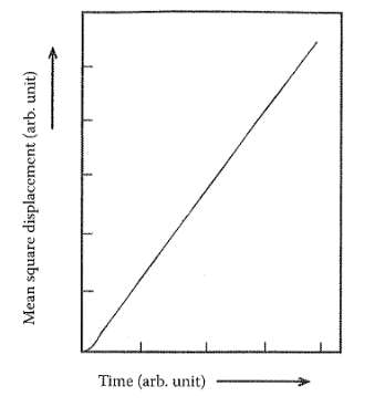
\(R^2(t)\) as a function of \(t\) is shown schematically in Fig. 16.1. We see that for short times it goes as \(t^2\). This is because for short times we can assume that the particle moves with almost constant velocity \(v\) and does not suffer any collision. Therefore,
\[ R=vt \]
or
\[ R^2=v^2t^2 \]
For long times, \(R^2(t)\) goes as \(t\). This is because for large \(t\) we can assume the particle to be a random walker for which \(R^2(t)\) varies linearly with \(t\). Thus, by calculating the slope of \(R^2(t)\) at large \(t\), the diffusion constant can be calculated from Equation Eq. 16.12.
Another important quantity is velocity autocorrelation function \(Z(t)\), which tells how the velocity \(\vec v(t)\) of a particle at time \(t\) is correlated with its velocity at time \(t=0\) on average, that is
\[ Z(t)=\left\langle\frac{1}{N}\sum_{i=1}^{N}\vec v_i(0)\cdot\vec v_i(t)\right\rangle \tag{16.13}\]
This is related to the diffusion constant by
\[ D=\frac{1}{3}\int_0^{\infty}Z(t)dt \tag{16.14}\]
Another important quantity, which one can get from the \(Z(t)\), is the phonon density of states, \(D(\omega)\), which can be obtained by taking the Fourier transform of \(Z(t)\) (Dickey and Paskin 1969)
\[ D(\omega)=c\int_0^{\infty}Z(t)\cos(\omega t)dt \tag{16.15}\]
where \(c\) is a constant.
16.4 First-Principles MD: Born-Oppenheimer Molecular Dynamics (BOMD)
To study ion dynamics using classical MD, one needs to know the phenomenological potential. For a given material, it is difficult to find a good potential. These are often obtained by hit and trial method and by fitting parameters to experimental data. Even if a good potential is known for a material, it has limited use. For example, it cannot be used in situations where electrons may play an important role.
In first-principles or ab initio MD, no such phenomenological potential is used and the forces on ions are calculated using quantum mechanical calculations. These calculations have no adjustable parameters. The only information one needs to know is the atomic numbers and masses of the atoms constituting the system.
Recall that in Chapter 2 , the total many-body wave function \(\phi\) could be decomposed by using the Born-Oppenheimer approximation as (see Equation <no-chapter-2-provided)
\[ \phi=\chi_i(\vec R)\psi_e(\vec r,\vec R) \tag{16.16}\]
where \(\chi_i\) is the wave function for ions and \(\psi_e\) is the wave function for electrons with ions at frozen positions \(\vec R\). \(\psi_e\) and \(\chi_i\) satisfy the following equations:
\[ \left[-\frac{\hbar^2}{2m_e}\sum_i\nabla_i^2+V_{ee}(\vec r)+V_{eI}(\vec r,\vec R)\right]\psi_e(\vec r,\vec R)=E_e(\vec R)\psi_e(\vec r,\vec R) \tag{16.17}\]
and
\[ \left[-\frac{\hbar^2}{2M}\sum_I\nabla_I^2+V_{II}(\vec R)+E_e(\vec R)\right]\chi_i(\vec R)=E\chi_i(\vec R) \tag{16.18}\]
where \(m_e\) is the mass of the electron and \(M\) is the mass of the ion. In the previous chapters, we have focused on solving Equation Eq. 16.17 using the DFT. Note that \(E_e\) is the total ground state electronic energy for the fixed position of ions and \(\psi_e(\vec r,\vec R)\) is the many-electron wave function. This problem was reduced to a one-electron problem using the DFT. We shall now focus on the solution of Equation Eq. 16.18 in which \(V_{II}+E_e\) provides the potential for ions.
We start with Ehrenfest’s theorem, which gives the following equations for the evolution of mean values of position and momentum operators for the ions (see, e.g., quantum mechanics by Merzbacher 1998).
\[ M\frac{d\langle\vec R\rangle}{dt}=\langle\vec P\rangle \tag{16.19}\]
and
\[ \frac{d\langle\vec P\rangle}{dt}=-\langle\vec\nabla(V_{II}(\vec R)+E_e(\vec R))\rangle \tag{16.20}\]
Substitution of Equation Eq. 16.19 into Equation Eq. 16.20 gives
\[ M\frac{d^2\langle\vec R\rangle}{dt^2}=-\langle\vec\nabla(V_{II}(\vec R)+E_e(\vec R))\rangle \tag{16.21}\]
Note that Equation Eq. 16.21 is valid only for the mean value of the position operator. However, we make an approximation here and identify the mean values with the positions of classical particles. This approximation is sometimes referred to as classical nuclei approximation. This is quite reasonable since the atoms have large mass and their de Broglie wavelength at room temperature is \(\sim 0.1\) Å, much smaller than the interatomic separations (of the order of few ångstroms). Thus, Equation Eq. 16.21 can be rewritten as
\[ M\frac{d^2\vec R}{dt^2}=-\vec\nabla\left(V_{II}(\vec R)+E_e(\vec R)\right) \tag{16.22}\]
We note that Equation Eq. 16.22 is very similar to Equation Eq. 16.2 of the classical MD, but now the potential is obtained from the first principles. Such MD in which the potential is obtained from the first principles is called first-principles or ab initio MD and the dynamics based on Equation Eq. 16.22 is known as the Born-Oppenheimer MD (BOMD). Such a dynamics can be based on the Hartree-Fock method or DFT, but here we shall assume that we are using DFT. In BOMD, the potential for ions is \(V_{II}(\vec R)+E_e(\vec R)\) and thus at each time step KS equations have to be solved and \(E_e(\vec R)\) has to be computed. Thus, in this dynamics, the electrons are always in the ground state and the dynamics are only due to the ions. In BOMD, the total energy of the system is a constant of motion which is
\[ E_{tot}=\frac{1}{2}\sum_i M_i\dot{\vec R}_i^2+V_{II}(\vec R)+E_e(\vec R) \tag{16.23}\]
16.5 First-Principles MD: Car-Parrinello Molecular Dynamics (CPMD)
As mentioned above, a first-principles MD can be based on Equation Eq. 16.22. To do this, we will have to calculate \(E_e(\vec R)\), which is the total energy of the electrons in the ground state corresponding to the fixed positions of the atoms. This means that at each step we will have to calculate the ground state of the system self-consistently, which could be computationally very time consuming. Car and Parrinello (1985) proposed an alternative which did not involve electronic self-consistency at each step and thus made the first-principles MD computationally very efficient.
To do this, they proposed a Lagrangian in which the single particle electronic orbitals \(\psi_i(\vec r,t)\) are also dynamical variables along with nuclear coordinates \(\vec R_i(t)\). The dynamics of nuclei is real while the dynamics of the orbitals is fictitious. This was a great idea which led to considerable savings in computational cost and made the first-principles MD possible. CPMD was first proposed by Car and Parrinello (1985) using the following Lagrangian:
\[ \begin{aligned} L=&\frac{1}{2}\sum_i M_i\dot{\vec R}_i^2+\sum_i\mu\int |\dot\psi_i(\vec r,t)|^2d^3r-E[\{\psi_i\},\{\vec R_i\}]\\ &+\sum_{ij}\Lambda_{ij}\left(\int\psi_i^*(\vec r,t)\psi_j(\vec r,t)d^3r-\delta_{ij}\right) \end{aligned} \tag{16.24}\]
where
\[ \begin{aligned} E[\{\psi_i\},\{\vec R_i\}]&=E_e(\vec R)+V_{II}(\vec R)\\ &=\sum_i^N\int\psi_i^*(\vec r,t)\left(-\frac{\hbar^2}{2m_e}\nabla^2\right)\psi_i(\vec r,t)d^3r\\ &+\int v(\vec r)n(\vec r)d^3r+\frac{1}{2}\iint\frac{e^2}{4\pi\varepsilon_0}\frac{n(\vec r)n(\vec r')}{|\vec r-\vec r'|}d^3r d^3r'\\ &+E_{xc}[n]+V_{II}(\vec R) \end{aligned} \tag{16.25}\]
where
\[ n(\vec r)=\sum_{i,\text{occupied}}|\psi_i(\vec r,t)|^2 \tag{16.26}\]
The first term in Equation Eq. 16.24 is the total kinetic energy of the atoms and the last term arises because of the constraint that the orbitals be orthonormal. In this term, \(\Lambda_{ij}\) are the Lagrange multipliers. Since the Lagrangian is real, the matrix \(\Lambda\) is Hermitian, that is \(\Lambda_{ij}=\Lambda_{ji}^*\). The second term was introduced by Car and Parrinello (1985) as a computational device and as such has no physical meaning. It represents a fictitious kinetic energy associated with the orbitals which are frequently referred to as electronic degrees of freedom. \(\mu\) is fictitious mass such that, in the limit \(\mu\to 0\), we get the true Lagrangian of the system.
Using Lagrangian (Eq. 16.24), equations of motions for the dynamical variables \(\{\vec R_i\}\) and \(\{\psi_i\}\) can be written as
\[ \frac{d}{dt}\left(\frac{\partial L}{\partial\dot{\vec R}_i}\right)=\frac{\partial L}{\partial\vec R_i} \tag{16.27}\]
and
\[ \frac{d}{dt}\left(\frac{\delta L}{\delta\dot\psi_i^*(\vec r,t)}\right)=\frac{\delta L}{\delta\psi_i^*(\vec r,t)} \tag{16.28}\]
Note that Equation Eq. 16.28 involves functional derivatives because the orbitals are not simple variables but are continuous scalar fields. From Equations Eq. 16.27 and Eq. 16.28, we get
\[ M\ddot{\vec R}_i=-\frac{\partial E[\{\psi_i\},\{\vec R_i\}]}{\partial\vec R_i} \tag{16.29}\]
and
\[ \mu\ddot\psi_i(\vec r,t)=-\frac{\delta E[\{\psi_i\},\{\vec R_i\}]}{\delta\psi_i^*(\vec r,t)}+\sum_j\Lambda_{ij}\psi_j(\vec r,t) \tag{16.30}\]
\[ =-H_{KS}\psi_i(\vec r,t)+\sum_j\Lambda_{ij}\psi_j(\vec r,t) \tag{16.31}\]
where
\[ H_{KS}=-\frac{\hbar^2}{2m_e}\nabla^2+v(\vec r)+v_{xc}(\vec r)+\int\frac{e^2}{4\pi\varepsilon_0}\frac{n(\vec r')}{|\vec r-\vec r'|}d^3r' \tag{16.32}\]
Equations Eq. 16.29 and Eq. 16.31 are the desired equations of motion for \(\{\vec R_i\}\) and \(\{\psi_i(\vec r,t)\}\). Note that while the dynamics of the ions is real, the dynamics of orbitals is fictitious and is introduced as a convenient computational tool to avoid costly solution of the KS equations at each time step as is the case in BOMD. Equation Eq. 16.30 tries to simulate the adiabatic evolution of KS orbitals on the Born-Oppenheimer (B-O) surface which is given by
\[ H_{KS}(t)\psi_i^{KS}(\vec r,t)=\varepsilon_i(t)\psi_i^{KS}(\vec r,t) \tag{16.33}\]
where time dependence of \(H_{KS}(t)\) comes from time dependence of the ionic coordinates. The dynamics generated by Equation Eq. 16.30 for the KS orbitals will be, in general, different from the adiabatic evolution of \(\psi_i^{KS}(\vec r,t)\) given by Equation Eq. 16.33. Thus, this scheme will work only if the wave functions obtained by Equation Eq. 16.31 remain close to the solutions of Equation Eq. 16.33. If one starts from an initial condition, when all the electrons are in the ground state (i.e., the system is on the B-O surface), from Equations Eq. 16.29 and Eq. 16.31, one can find the solution for \(\{\vec R_i\}\) and \(\{\psi_i(\vec r,t)\}\) at any later time by using algorithms such as the Verlet algorithm. Care should be taken so that the orbitals \(\{\psi_i(\vec r,t)\}\) are orthonormal to each other at each time step. This can be achieved by using the SHAKE algorithm discussed in Appendix. Note that subsequently time steps depend not solely on the electronic structure problem (Equation Eq. 16.33), but one simply updates the orbitals using Equation Eq. 16.31. Thus, the Car-Parrinello strategy results in tremendous savings in computational cost.
Now we shall prove that the eigenvalues of the matrix \(\Lambda\) are the single-particle energies of the KS equations. Assume that the left-hand side of Equation Eq. 16.31 is zero, that is, \(\ddot\psi_i=0\). This means that the forces on the orbitals are zero which would be the case when the electrons are in the ground state. Then Equation Eq. 16.31 reads as
\[ H_{KS}\psi_i=\sum_j\Lambda_{ij}\psi_j \]
or in matrix form
\[ \hat H_{KS}\psi=\Lambda\psi \tag{16.34}\]
Since matrix \(\Lambda\) is Hermitian, it can be diagonalized by a unitary matrix. Let \(U\) be the unitary matrix which diagonalizes it. Then,
\[ U^{-1}\hat H_{KS}U(U^{-1}\psi)=(U^{-1}\Lambda U)(U^{-1}\psi) \]
or
\[ \hat H_{KS}\psi'=\varepsilon'\psi' \tag{16.35}\]
where \(\varepsilon'\) is a diagonal matrix consisting of eigenvalues \(\varepsilon_i'\) and \(\hat H_{KS}\) and \(\psi'\) are transformed matrices under the unitary transformation. Now since \(\hat H_{KS}\) and \(H_{KS}\) are related by a unitary transformation, they have the same eigenvalues. Therefore, \(\varepsilon_i'\), that is, eigenvalues of matrix \(\Lambda\) can be interpreted as the KS eigenvalues.
An explicit expression for \(\Lambda_{ij}\) can be obtained by multiplying Equation Eq. 16.31 by \(\psi_j^*\) and then integrating,
\[ \Lambda_{ij}=H_{ij}^{KS}+\mu\int \dot\psi_i^*(\vec r,t)\dot\psi_j(\vec r,t)d^3r \tag{16.36}\]
where
\[ H_{ij}^{KS}=\int\psi_i^*(\vec r,t)H_{KS}\psi_j(\vec r,t)d^3r. \]
Equation Eq. 16.36 can be simplified by noting that \(H_{KS}\) and \(\Lambda\) are Hermitian, that is
\[ \begin{aligned} \Lambda_{ij}&=\frac{1}{2}(\Lambda_{ij}+\Lambda_{ji}^*)\\ &=H_{ij}^{KS}+\frac{1}{2}\mu\int\left(\dot\psi_i^*\dot\psi_j+\dot\psi_j^*\dot\psi_i\right)d^3r \end{aligned} \tag{16.37}\]
Let us differentiate the following orthonormality condition twice with respect to time, that is
\[ \int\psi_i^*\psi_jd^3r=\delta_{ij} \]
This gives
\[ \int(\ddot\psi_i^*\psi_j+\psi_i^*\ddot\psi_j)d^3r=-2\int\dot\psi_i^*\dot\psi_jd^3r. \]
Thus, we get
\[ \Lambda_{ij}=H_{ij}^{KS}-\mu\int\psi_i^*\ddot\psi_jd^3r \tag{16.38}\]
Although this equation is not useful for numerical calculation, this is the only form of the Lagrange multiplier matrix compatible with the equation of motion (Eq. 16.31).
The conserved quantity for Lagrangian (Eq. 16.24) is the total energy \(E_{tot}\) which is
\[ E_{tot}=\frac{1}{2}\sum_iM_i\dot{\vec R}_i^2+\sum_{i,\text{occupied}}\mu\int|\dot\psi_i|^2d^3r+E[\{\psi_i\},\{\vec R_i\}] \tag{16.39}\]
Note that the fictitious kinetic energy is included in \(E_{tot}\).
16.6 Comparison of the BOMD and CPMD
As mentioned earlier in BOMD, the dynamics are only due to the ions and the electrons are always in the ground state. Thus, there could be a use of relatively large time step for integration of motion compared to CPMD where the time step has to be chosen small as the electrons are also involved in the dynamics. However, in CPMD, the KS equations have to be solved only in the beginning while in BOMD one has to do it at each time step which may be very time consuming.
In BOMD, the electrons are always in the ground state as KS equations are solved at each time step. The CPMD avoids the need of solving the KS equations at each time step by using a fictitious dynamics of electrons. Thus, the Car-Parrinello scheme will work well if the electronic and nuclear dynamics stay very close to the instantaneous ground state, that is, the system is close to the B-O surface. This will happen if the exchange of energy between nuclear and electronic degrees of freedom is small. Thus, if there is a large energy gap between the highest occupied level (HOMO) and the lowest unoccupied level (LUMO), the scheme will generally work well. This is because if the gap is much larger than \(\hbar\omega\), where \(\omega\) is the typical vibrational frequency of atoms, the electrons will remain close to the ground state. There are nuclear and electronic degrees of freedom. Therefore, the electrons will remain close to the ground state assuming that the system was started from the ground state. If the gap is comparable to \(\hbar\omega\) or there is no gap, there will be an exchange of energy between nuclear and electronic degrees of freedom and the scheme will not work well. If the gap opens and closes periodically during the simulations, the scheme will also not work. The BOMD does not face this kind of problem.
16.7 Method of Steepest Descent
If one is not interested in the dynamics but only wants to find the energy minimum or the ground state geometry, the simplest method to use is the method of SD. In this method, one solves the following first-order differential equations instead of Equations Eq. 16.29 and Eq. 16.30 of CPMD.
\[ M_i\dot{\vec R}_i=-\frac{\partial E}{\partial\vec R_i} \tag{16.40}\]
\[ \mu\dot\psi_i=-\frac{\delta E}{\delta\psi_i^*}+\sum_j\Lambda_{ij}\psi_j \tag{16.41}\]
From Equation Eq. 16.40, one can see that once the energy minimum is attained, \(\dot{\vec R}_i=0\), that is, the nuclear coordinates do not change any further. Similarly, \(\dot\psi_i=0\) when the ground state of the system is attained. Solving Equations Eq. 16.40 and Eq. 16.41 together using the SD method is referred to as combined electron-ion minimization. Thus, the SD method is a very efficient way to find the energy minimum. Note that in the SD method, only the end product matters and time \(t\) does not have any physical significance. It is just a parameter or tool to achieve the end. The main drawback of the SD method is that one can get stuck in a local minimum and once one is stuck, there is no way of coming out of it.
The SD method can be used to solve Equation Eq. 16.41, that is, to solve the KS problem. This is frequently referred to as electron minimization. There are various other schemes in use, but we shall not discuss them here.
16.8 Simulated Annealing
The main drawback of the SD method to find the ground state configuration is that one can get trapped in a local minimum. The energy function \(E(\{\vec R_i(t)\})\) can have several local minima, but we are interested in the global minimum. The situation is schematically shown in Fig. 16.2, which shows a hypothetical energy function \(E(x)\) as function of some variable \(x\). This function has local minima at \(x_1\), \(x_2\), and has the global minimum at \(x_3\). We are interested in finding the global minimum.
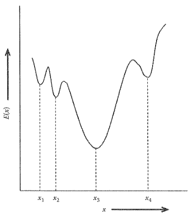
The problem of finding the global minimum of the energy function is the problem of nonlinear optimization encountered in several fields. In the current case, we have to minimize energy, which depends on several variables in a nonlinear fashion, and the minimization has to be done subject to certain constraints. One very interesting and powerful method to solve this kind of problem was suggested by Kirkpatrick et al. (1983). This method is known as simulated annealing, as it tries to mimic the natural process of solidification of liquids by slow cooling. The idea can be understood as follows. Suppose we consider a metal and heat it so that it melts and forms a liquid. At high temperatures in the liquid state, its atoms will move rapidly with respect to each other. As the liquid is slowly cooled, the atoms will move slower and slower. At certain temperature the liquid will solidify and if the cooling rate is slow enough, it may solidify in a crystalline state, which is the lowest state of energy. If one cools the liquid quickly or “quenches” it, the system may solidify in an amorphous or disordered state. Thus, by slow cooling or “annealing,” we can find the minimum energy state. This is the idea behind the simulated annealing.
Simulated annealing can be implemented either using the Metropolis algorithm or MD. When implemented using the MD, it is also referred to as dynamical simulated annealing. In the current case, when we want to study dynamics of ions, it is natural to implement simulated annealing using MD. It is implemented as follows:
Heat the system so that the system is in liquid state. This can be easily done by rescaling the velocities of atoms so that the temperature increases above the melting temperature.
Equilibrate the system for several thousand time steps. The idea is that all the atoms should move sufficiently far from their original positions.
Cool the system very slowly to temperature \(T=0\).
Note the position of atoms and the energy at \(T=0\).
Repeat steps 1 through 4 several times.
One hopes that by following the above steps one obtains the state of minimum energy. Note that in the simulated annealing method, the system can get out of the local minimum if it has sufficient kinetic energy. This was not possible in SD method, because as soon as the system reaches the minimum, it loses its kinetic energy.
16.9 Hellmann-Feynman Theorem
The Hellmann-Feynman theorem is used to calculate forces on the ions. From Equation Eq. 16.29, the force on the \(i\)th ion is
\[ \vec F_i=-\frac{\partial E}{\partial\vec R_i} \tag{16.42}\]
where
\[ E=E_e+V_{II} \]
is given by Equation Eq. 16.25.
Thus,
\[ \vec F_i=-\left[\frac{\partial E_e}{\partial\vec R_i}+\frac{\partial V_{II}}{\partial\vec R_i}\right]=\vec F_i^e+\vec F_i^I \tag{16.43}\]
\(E_e\) can be written as
\[ E_e=\langle\psi|H|\psi\rangle \tag{16.44}\]
where \(\psi\) is the many-electron wave function and \(H\) is the Hamiltonian of the system. \[ \begin{aligned} \frac{\partial E_e}{\partial\vec R_i} &= \frac{\partial}{\partial\vec R_i} \left(\langle\psi|H|\psi\rangle\right) \\ &= \left\langle\psi\left| \frac{\partial H}{\partial\vec R_i} \right|\psi\right\rangle + \left\langle \frac{\partial\psi}{\partial\vec R_i} \left|H\right|\psi \right\rangle \\ &\quad+ \left\langle \psi\left|H\right| \frac{\partial\psi}{\partial\vec R_i} \right\rangle \end{aligned} \tag{16.45}\]
If \(\psi\) is the eigenfunction of \(H\), then the last two terms of Equation Eq. 16.45 can be written as
\[ E_e\left\langle\frac{\partial\psi}{\partial\vec R_i}\middle|\psi\right\rangle+E_e\left\langle\psi\middle|\frac{\partial\psi}{\partial\vec R_i}\right\rangle =E_e\frac{\partial}{\partial\vec R_i}\langle\psi|\psi\rangle=0. \]
Thus,
\[ \vec F_i^e=-\frac{\partial E_e}{\partial\vec R_i}=-\left\langle\psi\left|\frac{\partial H}{\partial\vec R_i}\right|\psi\right\rangle \tag{16.46}\]
Thus, if \(\psi\) is the normalized eigenfunction of \(H\), \(\partial E_e/\partial\vec R_i\) is given by Equation Eq. 16.46. This statement is known as the Hellmann-Feynman theorem. If \(\psi\) is not normalized, Equations Eq. 16.44 and Eq. 16.45 can be expressed as
\[ E_e=\frac{\langle\psi|H|\psi\rangle}{\langle\psi|\psi\rangle} \tag{16.47}\]
and
\[ \vec F_i^e=-\frac{\partial E_e}{\partial\vec R_i}=-\frac{\left\langle\psi\left|\partial H/\partial\vec R_i\right|\psi\right\rangle}{\langle\psi|\psi\rangle} \tag{16.48}\]
This is because \(\partial/\partial\vec R_i\langle\psi|\psi\rangle=0\).
Let us look at the change in energy \(\delta E_e\) and the change in force \(\delta F_i^e\) due to a slight change in wave function by an amount \(\delta\psi\).
\[ \begin{aligned} \delta E_e &=\frac{\langle\psi+\delta\psi|H|\psi+\delta\psi\rangle}{\langle\psi+\delta\psi|\psi+\delta\psi\rangle}-\frac{\langle\psi|H|\psi\rangle}{\langle\psi|\psi\rangle}\\ &=\frac{\langle\psi|H|\delta\psi\rangle+\langle\delta\psi|H|\psi\rangle+\langle\delta\psi|H|\delta\psi\rangle}{\langle\psi|\psi\rangle}+O(\delta\psi^2)\\ &\quad -\frac{E_e(\langle\psi|\delta\psi\rangle+\langle\delta\psi|\psi\rangle)}{\langle\psi|\psi\rangle}+O(\delta\psi^2)\\ &=O(\delta\psi^2) \end{aligned} \]
or
\[ E_e=E_e^0+O(\delta\psi^2) \tag{16.49}\]
Thus, the change in energy is second order with respect to the change in wave function.
If the change in \(\delta\psi\) is of the same order as the change in \(\vec R_i\), then the change in the force is of first order with respect to the change in the wave function. Thus, the forces calculated using the Hellmann-Feynman theorem are more sensitive to the errors in the wave functions. Thus, it is easier to calculate an accurate total energy than to calculate an accurate force (see, e.g., Payne et al. 1992).
16.10 Calculation of Forces
The force acting on \(\ell\)th ion is given by Equation Eq. 16.29, which is
\[ \vec F_\ell=-\frac{\partial E[\{\psi_i\},\{\vec R_i\}]}{\partial\vec R_\ell} \tag{16.50}\]
where \(E\) is given by
\[ \begin{aligned} E=&\sum_i\int\psi_i^*(\vec r)\left(-\frac{\hbar^2}{2m_e}\nabla^2\right)\psi_i(\vec r)d^3r\\ &+\int v(\vec r)n(\vec r)d^3r+/frac{1}{2}\iint\frac{e^2}{4\pi\varepsilon_0}\frac{n(\vec r)n(\vec r')}{|\vec r-\vec r'|}d^3r d^3r'\\ &+E_{xc}[n]+V_{II}(\vec R) \end{aligned} \tag{16.51}\]
The calculation of forces is the most time-consuming part of the MD calculation. This calculation can be speeded up by directly calculating forces on ions rather than first calculating \(E\) and then numerically differentiating it. The Hellmann-Feynman theorem in the form of Equation Eq. 16.46 is not very useful, as \(\psi\) appearing in this equation is the many-electron wave function. What we would like is an expression for the force in terms of single-particle orbitals \(\psi_i\) or one electron charge density \(n(\vec r)\).
To accomplish this, let us substitute Equation Eq. 16.51 into Equation Eq. 16.50 to get
\[ \vec F_\ell=-\frac{\partial}{\partial\vec R_\ell}\left[E_{kin}+E_{xc}+E_H+\int v(\vec r)n(\vec r)d^3r\right]-\frac{\partial}{\partial\vec R_\ell}V_{II}(\vec R) \tag{16.52}\]
We also know that \(\psi_i(\vec r)\) satisfies the KS equations
\[ \left[-\frac{\hbar^2}{2m_e}\nabla^2+v(\vec r)+\int\frac{e^2}{4\pi\varepsilon_0}\frac{n(\vec r')}{|\vec r-\vec r'|}d^3r'+\frac{\delta E_{xc}}{\delta n(\vec r)}\right]\psi_i(\vec r)=\varepsilon_i\psi_i(\vec r) \tag{16.53}\]
Note that \(\psi_i(\vec r)\) and \(\varepsilon_i\) depend on atomic positions \(\vec R_i\).
Let us now evaluate various terms in Equation Eq. 16.52. The first term gives
\[ -\frac{\partial E_{kin}}{\partial\vec R_\ell} =-\sum_i\int\left[\frac{\partial\psi_i^*}{\partial\vec R_\ell}\left(-\frac{\hbar^2}{2m_e}\nabla^2\right)\psi_i+\psi_i^*\left(-\frac{\hbar^2}{2m_e}\nabla^2\right)\frac{\partial\psi_i}{\partial\vec R_\ell}\right]d^3r \tag{16.54}\]
The second term gives
\[ -\frac{\partial E_{xc}[n]}{\partial\vec R_\ell}=-\int\frac{\delta E_{xc}[n]}{\delta n(\vec r)}\frac{\partial n(\vec r)}{\partial\vec R_\ell}d^3r \tag{16.55}\]
The third term gives
\[ \begin{aligned} -\frac{\partial E_H}{\partial\vec R_\ell} &=-\left[\frac{1}{2}\iint\frac{e^2}{4\pi\varepsilon_0}\frac{n(\vec r)}{|\vec r-\vec r'|}\frac{\partial n(\vec r')}{\partial\vec R_\ell}d^3r d^3r'\right.\\ &\left.\quad+\frac{1}{2}\iint\frac{e^2}{4\pi\varepsilon_0}\frac{\partial n(\vec r)}{\partial\vec R_\ell}\frac{n(\vec r')}{|\vec r-\vec r'|}d^3r d^3r'\right]\\ &=-\iint\frac{e^2}{4\pi\varepsilon_0}\frac{n(\vec r')}{|\vec r-\vec r'|}\frac{\partial n(\vec r)}{\partial\vec R_\ell}d^3r d^3r' \end{aligned} \tag{16.56}\]
The fourth term in Equation Eq. 16.52 gives
\[ -\int\left[\frac{\partial v(\vec r)}{\partial\vec R_\ell}n(\vec r)+v(\vec r)\frac{\partial n(\vec r)}{\partial\vec R_\ell}\right]d^3r \tag{16.57}\]
The last term gives
\[ \begin{aligned} -\frac{\partial}{\partial\vec R_\ell}V_{II}(\vec R) &=-\frac{\partial}{\partial\vec R_\ell}\frac{1}{2}\sum_{i\ne j}\frac{1}{4\pi\varepsilon_0}\frac{Z_iZ_je^2}{|\vec R_i-\vec R_j|}\\ &=-\frac{1}{2}\sum_{j\ne\ell}\frac{1}{4\pi\varepsilon_0}\frac{Z_\ell Z_je^2}{|\vec R_\ell-\vec R_j|^3}(\vec R_j-\vec R_\ell)\\ &\quad+\frac{1}{2}\sum_{i\ne\ell}\frac{1}{4\pi\varepsilon_0}\frac{Z_iZ_\ell e^2}{|\vec R_i-\vec R_\ell|^3}(\vec R_i-\vec R_\ell)\\ &=\sum_{j\ne\ell}\frac{1}{4\pi\varepsilon_0}\frac{Z_\ell Z_je^2}{|\vec R_\ell-\vec R_j|^3}(\vec R_\ell-\vec R_j) \end{aligned} \tag{16.58}\]
Also we know that
\[ n(\vec r)=\sum_i\psi_i^*(\vec r)\psi_i(\vec r) \tag{16.59}\]
so that
\[ \frac{\partial n(\vec r)}{\partial\vec R_\ell}=\sum_i\left[\frac{\partial\psi_i^*(\vec r)}{\partial\vec R_\ell}\psi_i(\vec r)+\psi_i^*(\vec r)\frac{\partial\psi_i(\vec r)}{\partial\vec R_\ell}\right] \tag{16.60}\]
Substituting Equations Eq. 16.53 through Eq. 16.60 into Equation Eq. 16.52, we get
\[ \begin{aligned} \vec F_\ell=&\sum_{j\ne\ell}\frac{1}{4\pi\varepsilon_0}\frac{Z_\ell Z_je^2}{|\vec R_\ell-\vec R_j|^3}(\vec R_\ell-\vec R_j)-\int\frac{\partial v(\vec r)}{\partial\vec R_\ell}n(\vec r)d^3r\\ &-\sum_i\int\frac{\partial\psi_i^*}{\partial\vec R_\ell}\left[-\frac{\hbar^2}{2m_e}\nabla^2+\frac{\delta E_{xc}}{\delta n(\vec r)}+\int\frac{e^2}{4\pi\varepsilon_0}\frac{n(\vec r')}{|\vec r-\vec r'|}d^3r'+v(\vec r)\right]\psi_i d^3r\\ &-\sum_i\int\psi_i^*\left[-\frac{\hbar^2}{2m_e}\nabla^2+\frac{\delta E_{xc}}{\delta n(\vec r)}+\int\frac{e^2}{4\pi\varepsilon_0}\frac{n(\vec r')}{|\vec r-\vec r'|}d^3r'+v(\vec r)\right]\frac{\partial\psi_i}{\partial\vec R_\ell}d^3r \end{aligned} \tag{16.61}\]
Using Equation Eq. 16.53 the last two terms of Equation Eq. 16.61 (terms in the curly brackets) can be written as
\[ -\sum_i\varepsilon_i\int\left[\frac{\partial\psi_i^*}{\partial\vec R_\ell}\psi_i+\psi_i^*\frac{\partial\psi_i}{\partial\vec R_\ell}\right]d^3r =-\sum_i\varepsilon_i\frac{\partial}{\partial\vec R_\ell}\int\psi_i^*\psi_i d^3r=0 \tag{16.62}\]
Thus, the force on \(\ell\)th atom can be given as
\[ \vec F_\ell=\sum_{j\ne\ell}\frac{1}{4\pi\varepsilon_0}\frac{Z_\ell Z_je^2}{|\vec R_\ell-\vec R_j|^3}(\vec R_\ell-\vec R_j)-\int\frac{\partial v(\vec r)}{\partial\vec R_\ell}n(\vec r)d^3r \tag{16.63}\]
This is the Hellmann-Feynman theorem in terms of single particle charge density or single particle orbitals. This theorem greatly simplifies the calculation of forces on ions. It should be emphasized that this theorem is applicable only if the electronic wave functions are eigenstates of the KS Hamiltonian as we have assumed in Equation Eq. 16.62. If this is not so, then the terms in curly brackets in Equation Eq. 16.61 are not zero. Thus, in general, we should write the total force on ions as a sum of two terms as
\[ \vec F_\ell=\vec F_\ell^{HF}+\vec F_\ell^v \tag{16.64}\]
where \(\vec F_\ell^{HF}\) is the Hellmann-Feynman force given by Equation Eq. 16.63 and \(\vec F_\ell^v\) is the term in curly brackets in Equation Eq. 16.61 and we refer to it as variational force. This force will be present if the electronic wave functions are not the eigenstates of the KS Hamiltonian or if the wave function has been expanded using an incomplete basis set as we shall see below.
Since the two terms in the curly brackets in Equation Eq. 16.61 are complex conjugates, we can write \(\vec F_\ell^v\) as
\[ \vec F_\ell^v=-2\operatorname{Re}\sum_i\int\frac{\partial\psi_i^*}{\partial\vec R_\ell}\left[-\frac{\hbar^2}{2m_e}\nabla^2+v_{eff}(\vec r)\right]\psi_i d^3r \tag{16.65}\]
where Re denotes the real part and
\[ v_{eff}[n]=\frac{\delta E_{xc}}{\delta n}+\int\frac{e^2}{4\pi\varepsilon_0}\frac{n(\vec r')}{|\vec r-\vec r'|}d^3r'+v(\vec r) \tag{16.66}\]
Equation Eq. 16.65 can be written as
\[ \vec F_\ell^v=-2\operatorname{Re}\sum_j\int\frac{\partial\psi_j^*}{\partial\vec R_\ell}\left[-\frac{\hbar^2}{2m_e}\nabla^2+v_{eff}[n]-\varepsilon_j\right]\psi_jd^3r \tag{16.67}\]
where we have used
\[ \frac{\partial}{\partial\vec R_\ell}\left(\varepsilon_j\int\psi_j^*\psi_jd^3r\right)=0. \]
Recall that the KS equations are solved self-consistently. That is, one starts with a charge density \(\bar n(\vec r)\), constructs potential \(v_{eff}[\bar n]\), and then obtains charge density by solving KS equations. The process is repeated until self-consistency is achieved, that is, output potential and input potentials are the same within some tolerance. Although for most purposes, this may yield the desired accuracy, yet the self-consistency is never exact. Thus, if the calculation is not fully self-consistent, the wave functions are calculated for different potential \(v_{eff}[\bar n]\) related to the previous iteration. We add and subtract this potential in Equation Eq. 16.67, which gives
\[ \begin{aligned} \vec F_\ell^v=&-2\operatorname{Re}\sum_j\int\frac{\partial\psi_j^*}{\partial\vec R_\ell}\left[-\frac{\hbar^2}{2m_e}\nabla^2+v_{eff}[\bar n]-\varepsilon_j\right]\psi_jd^3r\\ &-2\operatorname{Re}\sum_j\int\frac{\partial\psi_j^*}{\partial\vec R_\ell}\left[v_{eff}[n]-v_{eff}[\bar n]\right]\psi_jd^3r \end{aligned} \tag{16.68}\]
\[ =\vec F_\ell^{IBS}+\vec F_\ell^{NSC} \tag{16.69}\]
The second term in Equation Eq. 16.69, \(\vec F^{NSC}\), is a measure of nonself-consistency in the solution of the KS equation. To make this term small, it is important to bring the calculation very close to self-consistency. If this is achieved, \(\vec F^{NSC}\) can be made arbitrarily small.
The first term \(\vec F^{IBS}\) in Equation Eq. 16.69 arises due to the use of incomplete basis set and is usually referred to as the Pulay force (Pulay 1969, Srivastava and Weaire 1987, Martin 2004). This term includes the single particle equations, which should have been solved in the last but one iteration. But such a solution is usually not exact, because a finite, \(N_i\) dimensional basis set has been used in expanding the wave function
\[ \psi_i(\vec r,\vec R)=\sum_{j=1}^{N_b}C_{ij}(\vec R)\phi_j(\vec r,\vec R) \tag{16.70}\]
where \(\vec R\) denotes the ionic coordinates \(\{\vec R_i\}\) and \(\phi_j(\vec r,\vec R)\) the basis functions. Substituting this in the first term of Equation Eq. 16.68, we get
\[ \begin{aligned} \vec F_\ell^{IBS}=&-2\operatorname{Re}\sum_{i=1}^{N}\sum_{j=1}^{N_b}\sum_{j'=1}^{N_b}\int\frac{\partial C_{ij'}^*\phi_{j'}^*}{\partial\vec R_\ell}\left[-\frac{\hbar^2}{2m_e}\nabla^2+v_{eff}[\bar n]-\varepsilon_i\right]C_{ij}\phi_jd^3r\\ =&-2\operatorname{Re}\sum_{i=1}^{N}\sum_{j=1}^{N_b}\sum_{j'=1}^{N_b}\int C_{ij'}^*\frac{\partial\phi_{j'}^*}{\partial\vec R_\ell}\left[-\frac{\hbar^2}{2m_e}\nabla^2+v_{eff}[\bar n]-\varepsilon_i\right]C_{ij}\phi_jd^3r \end{aligned} \tag{16.71}\]
Note that the actual secular equation, which one solves, is
\[ \sum_{j=1}^{N_b}\int\phi_{j'}^*\left[-\frac{\hbar^2}{2m_e}\nabla^2+v_{eff}[\bar n]-\varepsilon_i\right]C_{ij}\phi_jd^3r=0 \tag{16.72}\]
Because of this, the first term in Equation Eq. 16.71 becomes zero but the second term will be usually different from zero. Thus,
\[ \vec F_\ell^{IBS}=-2\operatorname{Re}\sum_{i=1}^{N}\sum_{j=1}^{N_b}\sum_{j'=1}^{N_b}C_{ij'}^*C_{ij}\int\frac{\partial\phi_{j'}^*}{\partial\vec R_\ell}\left[-\frac{\hbar^2}{2m_e}\nabla^2+v_{eff}[\bar n]-\varepsilon_i\right]\phi_jd^3r \tag{16.73}\]
Thus, if the basis set depends on the ionic position as is the case with LMTO or LCAO basis sets, the Pulay forces will be finite. However, for the plane wave basis set, which does not depend on ionic coordinates, we see from Equation Eq. 16.73 that the Pulay forces are zero. This is a great advantage of using the plane wave basis set.
Note that we have proved Equation Eq. 16.73 using the DFT and using all electron potential \(v(\vec r)\). This proof can also be extended for pseudopotential.
16.11 Applications of the First-Principles MD
The first-principles MD has been applied to study various systems such as atomic clusters, nanowires, amorphous systems, surfaces and interfaces, biomolecules, water and nonaqueous liquids, chemical reactions, catalysis, and so on. Some of these applications will be discussed in subsequent chapters of the book. For more information, we refer to the excellent review articles by Car and Parrinello (1989), Payne et al. (1992), and Remler and Madden (1990) and the books by Kohanoff (2006) and Marx and Hutter (2009).
16.12 Exercises
Show that the mean-squared displacement \(R^2(t)\) in three dimensions, in the limit of \(t\) tending to infinity, can be shown as
\[ R^2(t)=6Dt \quad t\to\infty \quad (3\ \text{dimensions}) \]
Show that the diffusion constant \(D\) can be written as
\[ D=\frac{1}{3}\int_0^{\infty}Z(t)dt \]
Show that the phonon density of states \(D(\omega)\) can be obtained by taking Fourier transform of \(Z(t)\)
\[ D(\omega)=c\int_0^{\infty}Z(t)\cos(\omega t)dt \]
where \(c\) is a constant.
Calculate the mean-squared displacement \(R^2(t)\) for a system of particles interacting via Lennard-Jones potential given by
\[ V(r)=4\varepsilon\left[\left(\frac{\sigma}{r}\right)^{12}-\left(\frac{\sigma}{r}\right)^6\right] \]
where \(r\) is the interatomic distance and \(\varepsilon\) and \(\sigma\) are parameters. Take the values of the parameters corresponding to argon (see, e.g., Rahman 1964) and check that the mean-squared displacement \(R^2(t)\) has correct behavior as time \(t\) tends to zero and infinity.
Prove that
\[ \begin{aligned} \Lambda_{ij}&=H_{ij}^{KS}+\mu\int\dot\psi_i^*(\vec r,t)\dot\psi_j(\vec r,t)d^3r\\ &=H_{ij}^{KS}-\mu\int\psi_i^*\ddot\psi_jd^3r. \end{aligned} \]
Show that for a plane wave basis set the Pulay force is zero.
Find bond length and vibrational frequency of a silicon dimer using the CPMD and BOMD. Use one of the MD codes listed in Appendix A. Take a large cubical supercell of length about 10 Å and use the method of SD for finding bond length. For finding the vibrational frequency, displace one of the atoms by a small amount \(\sim 0.01\) Å and calculate time period of one oscillation using CPMD or BOMD. Compare the results obtained by CPMD and BOMD.
Calculate the structure of a silicon trimer using the simulated annealing. Use a large supercell and one of the MD codes listed in Appendix A. Heat the system upto 1500 K and then slowly cool it to 300 K. Below 300 K, you may use the method of SD to get the structure.
16.13 Further Reading
Haile J. M. 1997. Molecular Dynamics Simulation: Elementary Methods. New York: John Wiley & Sons.
Kohanoff J. 2006. Electronic Structure Methods for Solids and Molecules. Cambridge: Cambridge University Press.