6 Hydrogen atom
6.1 Schrödinger Equation in Spherical Coordinates
The generalization to three dimensions is straightforward. Schrödinger’s equation says
\[ i\hbar\frac{\partial\Psi}{\partial t} = H\Psi, \tag{6.1}\]
the Hamiltonian operator \(H\) is obtained from the classical energy
\[ \frac{1}{2}mv^2 + V = \frac{1}{2m}(p_x^2 + p_y^2 + p_z^2) + V \]
by the standard prescription (applied now to \(y\) and \(z\), as well as \(x\)):
\[ p_x \to \frac{\hbar}{i}\frac{\partial}{\partial x}, \quad p_y \to \frac{\hbar}{i}\frac{\partial}{\partial y}, \quad p_z \to \frac{\hbar}{i}\frac{\partial}{\partial z}, \tag{6.2}\]
or
\[ \boxed{\mathbf{p} \to \frac{\hbar}{i}\nabla,} \tag{6.3}\]
for short. Thus
\[ \boxed{i\hbar\frac{\partial\Psi}{\partial t} = -\frac{\hbar^2}{2m}\nabla^2\Psi + V\Psi,} \tag{6.4}\]
where
\[ \nabla^2 \equiv \frac{\partial^2}{\partial x^2} + \frac{\partial^2}{\partial y^2} + \frac{\partial^2}{\partial z^2} \tag{6.5}\]
is the Laplacian, in Cartesian coordinates.
The potential energy \(V\) and the wave function \(\Psi\) are now functions of \(\mathbf{r} = (x,y,z)\) and \(t\). The probability of finding the particle in the infinitesimal volume \(d^3\mathbf{r} = dx\,dy\,dz\) is \(|\Psi(\mathbf{r},t)|^2\,d^3\mathbf{r}\), and the normalization condition reads
\[ \int|\Psi|^2\,d^3\mathbf{r} = 1, \tag{6.6}\]
with the integral taken over all space. If the potential is independent of time, there will be a complete set of stationary states,
\[ \Psi_n(\mathbf{r},t) = \psi_n(\mathbf{r})e^{-iE_nt/\hbar}, \tag{6.7}\]
where the spatial wave function \(\psi_n\) satisfies the time-independent Schrödinger equation:
\[ \boxed{-\frac{\hbar^2}{2m}\nabla^2\psi + V\psi = E\psi.} \tag{6.8}\]
The general solution to the (time-dependent) Schrödinger equation is
\[ \Psi(\mathbf{r},t) = \sum_n c_n\psi_n(\mathbf{r})e^{-iE_nt/\hbar}, \tag{6.9}\]
with the constants \(c_n\) determined by the initial wave function, \(\Psi(\mathbf{r},0)\), in the usual way. (If the potential admits continuum states, then the sum in Eq. 6.9 becomes an integral.)
- Work out all of the canonical commutation relations for components of the operators \(\mathbf{r}\) and \(\mathbf{p}\): \([x,y]\), \([x,p_y]\), \([x,p_x]\), \([p_y,p_z]\), and so on. Answer: \[ [r_i,p_j] = -[p_i,r_j] = i\hbar\delta_{ij}, \quad [r_i,r_j] = [p_i,p_j] = 0, \tag{6.10}\]
where the indices stand for \(x\), \(y\), or \(z\), and \(r_x = x\), \(r_y = y\), \(r_z = z\).
Confirm Ehrenfest’s theorem for 3-dimensions: \[ \frac{d}{dt}\langle\mathbf{r}\rangle = \frac{1}{m}\langle\mathbf{p}\rangle, \qquad\text{and}\qquad \frac{d}{dt}\langle\mathbf{p}\rangle = \langle-\nabla V\rangle. \tag{6.11}\] (Each of these, of course, stands for three equations — one for each component.) Hint: First check that Equation 3.71 is valid in three dimensions.
Formulate Heisenberg’s uncertainty principle in three dimensions.” collapse=true Answer:
\[ \sigma_x\sigma_{p_x} \geq \hbar/2, \quad \sigma_y\sigma_{p_y} \geq \hbar/2, \quad \sigma_z\sigma_{p_z} \geq \hbar/2, \tag{6.12}\]
but there is no restriction on, say, \(\sigma_x\sigma_{p_y}\).
6.1.1 Separation of Variables
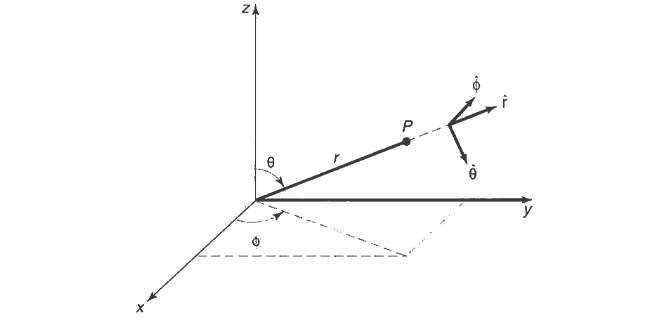
Typically, the potential is a function only of the distance from the origin. In that case it is natural to adopt spherical coordinates, \((r,\theta,\phi)\) (see Fig. 6.1). In spherical coordinates the Laplacian takes the form
\[ \nabla^2 = \frac{1}{r^2}\frac{\partial}{\partial r} \!\left(r^2\frac{\partial}{\partial r}\right) + \frac{1}{r^2\sin\theta}\frac{\partial}{\partial\theta} \!\left(\sin\theta\frac{\partial}{\partial\theta}\right) + \frac{1}{r^2\sin^2\theta} \frac{\partial^2}{\partial\phi^2}. \tag{6.13}\]
In spherical coordinates, then, the time-independent Schrödinger equation reads
\[ \begin{aligned} -\frac{\hbar^2}{2m}\Bigg[ &\frac{1}{r^2}\frac{\partial}{\partial r} \!\left(r^2\frac{\partial\psi}{\partial r}\right) \\[6pt] &+ \frac{1}{r^2\sin\theta}\frac{\partial}{\partial\theta} \!\left(\sin\theta\frac{\partial\psi}{\partial\theta}\right) \\[6pt] &+ \frac{1}{r^2\sin^2\theta} \frac{\partial^2\psi}{\partial\phi^2} \Bigg] + V\psi = E\psi. \end{aligned} \tag{6.14}\] We begin by looking for solutions that are separable into products:
\[ \psi(r,\theta,\phi) = R(r)\,Y(\theta,\phi). \tag{6.15}\]
Use separation of variables in Cartesian coordinates to solve the infinite cubical well (or “particle in a box”):
\[ V(x,y,z) = \begin{cases} 0, & \text{if } x,\,y,\,z \text{ are all between } 0 \text{ and } a;\\ \infty, & \text{otherwise.} \end{cases} \]
(a) Find the stationary states, and the corresponding energies.
(b) Call the distinct energies \(E_1, E_2, E_3, \ldots\), in order of increasing energy. Find \(E_1, E_2, E_3, E_4, E_5\), and \(E_6\). Determine their degeneracies (that is, the number of different states that share the same energy). Comment: In one dimension degenerate bound states do not occur , but in three dimensions they are very common.
(c) What is the degeneracy of \(E_{14}\), and why is this case interesting?
6.1.2 The Angular Equation
Eq. 6.17 determines the dependence of \(\psi\) on \(\theta\) and \(\phi\); multiplying by \(Y\sin^2\theta\), it becomes:
\[ \sin\theta\frac{\partial}{\partial\theta}\!\left(\sin\theta\frac{\partial Y}{\partial\theta}\right) + \frac{\partial^2 Y}{\partial\phi^2} = -l(l+1)\sin^2\theta\, Y. \tag{6.18}\]
You might recognize this equation — it occurs in the solution to Laplace’s equation in classical electrodynamics. As always, we try separation of variables:
\[ Y(\theta,\phi) = \Theta(\theta)\,\Phi(\phi). \tag{6.19}\]
Plugging this in and dividing by \(\Theta\Phi\), we find:
\[ \left\{\frac{1}{\Theta}\!\left[\sin\theta\frac{d}{d\theta}\!\left(\sin\theta\frac{d\Theta}{d\theta}\right)\right] + l(l+1)\sin^2\theta\right\} + \frac{1}{\Phi}\frac{d^2\Phi}{d\phi^2} = 0. \]
The first term is a function only of \(\theta\), and the second is a function only of \(\phi\), so each must be a constant. Calling the separation constant \(m^2\):
\[ \frac{1}{\Theta}\!\left[\sin\theta\frac{d}{d\theta}\!\left(\sin\theta\frac{d\Theta}{d\theta}\right)\right] + l(l+1)\sin^2\theta = m^2, \tag{6.20}\]
\[ \frac{1}{\Phi}\frac{d^2\Phi}{d\phi^2} = -m^2. \tag{6.21}\]
The \(\phi\) Equation
The \(\phi\) equation is easy:
\[ \frac{d^2\Phi}{d\phi^2} = -m^2\Phi \implies \Phi(\phi) = e^{im\phi}. \tag{6.22}\] Actually, there are two solutions: \(\exp(im\phi)\) and \(\exp(-im\phi)\), but we’ll cover the latter by allowing \(m\) to run negative. There could also be a constant factor in front, but we might as well absorb that into \(\Theta\). Incidentally, in electrodynamics we would write the azimuthal function \((\Phi)\) in terms of sines and cosines, instead of exponentials, because electric potentials must be real. In quantum mechanics there is no such constraint, and the exponentials are a lot easier to work with. Now, when \(\phi\) advances by \(2\pi\), we return to the same point in space (see Fig. 6.1), so it is natural to require that \[ \Phi(\phi+2\pi) = \Phi(\phi). \tag{6.23}\]
This means \(\exp(2\pi im) = 1\), from which it follows that \(m\) must be an integer:
\[ m = 0,\,\pm 1,\,\pm 2,\,\ldots \tag{6.24}\]
The \(\theta\) Equation
The \(\theta\) equation,
\[ \sin\theta\frac{d}{d\theta}\!\left(\sin\theta\frac{d\Theta}{d\theta}\right) + \bigl[l(l+1)\sin^2\theta - m^2\bigr]\Theta = 0, \tag{6.25}\]
is not so simple. The solution is
\[ \Theta(\theta) = A\,P_l^m(\cos\theta), \tag{6.26}\]
where \(P_l^m\) is the associated Legendre function, defined by
\[ P_l^m(x) \equiv (1-x^2)^{|m|/2}\!\left(\frac{d}{dx}\right)^{\!|m|}P_l(x), \tag{6.27}\]
and \(P_l(x)\) is the \(l\)th Legendre polynomial, defined by the Rodrigues formula:
\[ P_l(x) \equiv \frac{1}{2^l l!}\left(\frac{d}{dx}\right)^{\!l}(x^2-1)^l. \tag{6.28}\]
For example,
\[ P_0(x) = 1, \qquad P_1(x) = \frac{1}{2}\frac{d}{dx}(x^2-1) = x, \]
\[ P_2(x) = \frac{1}{4\cdot 2}\left(\frac{d}{dx}\right)^2(x^2-1)^2 = \frac{1}{2}(3x^2-1), \]
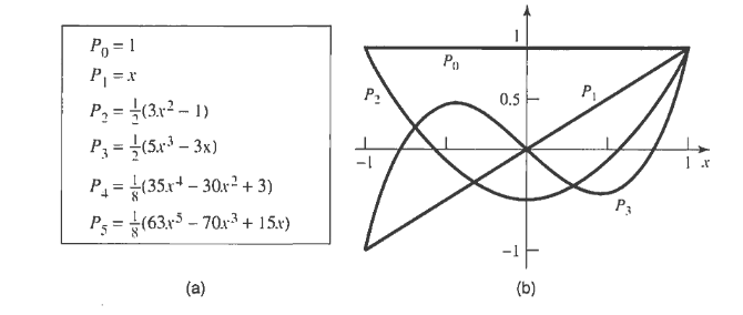
and so on. The first few Legendre polynomials are listed in Table 6.1.
Notice that \(l\) must be a nonnegative integer, for the Rodrigues formula to make any sense; moreover, if \(|m|>l\), then Eq. 6.27 says \(P_l^m = 0\). For any given \(l\), then, there are \((2l+1)\) possible values of \(m\):
\[ l = 0,\,1,\,2,\,\ldots;\qquad m = -l,\,-l+1,\,\ldots,\,-1,\,0,\,1,\,\ldots,\,l-1,\,l. \tag{6.29}\]
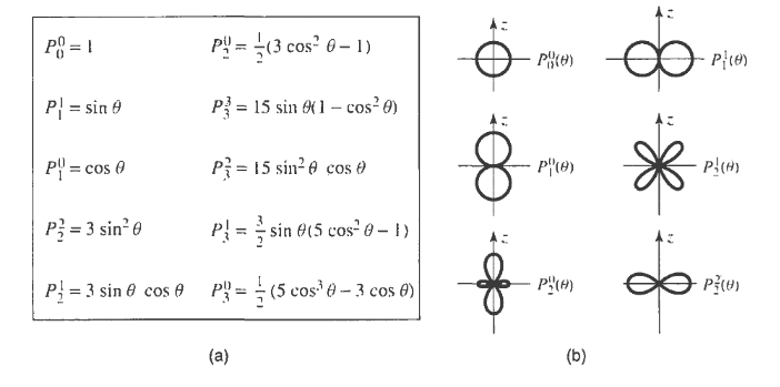
Some associated Legendre functions of \(\cos\theta\) are listed in Table 6.2.
The volume element in spherical coordinates is
\[ d^3\mathbf{r} = r^2\sin\theta\,dr\,d\theta\,d\phi, \tag{6.30}\]
so the normalization condition (Eq. 6.6) becomes
\[ \int|R|^2 r^2\,dr \int|Y|^2\sin\theta\,d\theta\,d\phi = 1. \]
It is convenient to normalize \(R\) and \(Y\) separately:
\[ \int_0^\infty |R|^2 r^2\,dr = 1 \qquad\text{and}\qquad \int_0^{2\pi}\!\int_0^\pi |Y|^2\sin\theta\,d\theta\,d\phi = 1. \tag{6.31}\]
Spherical Harmonics
The normalized angular wave functions are called spherical harmonics:
\[ \boxed{Y_l^m(\theta,\phi) = \epsilon\sqrt{\frac{(2l+1)}{4\pi}\frac{(l-|m|)!}{(l+|m|)!}}\,e^{im\phi}\,P_l^m(\cos\theta),} \tag{6.32}\]
where \(\epsilon = (-1)^m\) for \(m\geq 0\) and \(\epsilon=1\) for \(m\leq 0\). They are automatically orthogonal:
\[ \int_0^{2\pi}\!\int_0^\pi\bigl[Y_l^m(\theta,\phi)\bigr]^*\bigl[Y_{l'}^{m'}(\theta,\phi)\bigr]\sin\theta\,d\theta\,d\phi = \delta_{ll'}\delta_{mm'}. \tag{6.33}\]
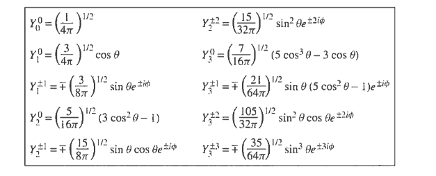
In Table 6.3 I have listed the first few spherical harmonics.
For historical reasons, \(l\) is called the azimuthal quantum number, and \(m\) the magnetic quantum number.
| \(l\) | Spectroscopic label |
|---|---|
| 0 | \(s\) |
| 1 | \(p\) |
| 2 | \(d\) |
| 3 | \(f\) |
Show that \[ \Theta(\theta) = A\ln[\tan(\theta/2)] \]
satisfies the \(\theta\) equation (Eq. 6.25), for \(l=m=0\). This is the unacceptable “second solution” — what’s wrong with it?
Starting from the Rodrigues formula, derive the orthonormality condition for Legendre polynomials:
\[ \int_{-1}^1 P_l(x)\,P_{l'}(x)\,dx = \left(\frac{2}{2l+1}\right)\delta_{ll'}. \tag{6.34}\]
Hint: Use integration by parts.
6.1.3 The Radial Equation
Notice that the angular part of the wave function, \(Y(\theta,\phi)\), is the same for all spherically symmetric potentials; the actual shape of the potential, \(V(r)\), affects only the radial part of the wave function, \(R(r)\), which is determined by Eq. 6.16:
\[ \frac{d}{dr}\!\left(r^2\frac{dR}{dr}\right) - \frac{2mr^2}{\hbar^2}[V(r)-E]R = l(l+1)R. \tag{6.35}\]
This equation simplifies if we change variables: Let
\[ u(r) \equiv r\,R(r), \tag{6.36}\]
so that \(R = u/r\), \(dR/dr = [r(du/dr)-u]/r^2\), \((d/dr)[r^2(dR/dr)] = r\,d^2u/dr^2\), and hence
\[ \boxed{-\frac{\hbar^2}{2m}\frac{d^2u}{dr^2} + \left[V + \frac{\hbar^2}{2m}\frac{l(l+1)}{r^2}\right]u = Eu.} \tag{6.37}\]
This is called the radial equation; it is identical in form to the one-dimensional Schrödinger equation , except that the effective potential,
\[ V_{\text{eff}} = V + \frac{\hbar^2}{2m}\frac{l(l+1)}{r^2}, \tag{6.38}\]
The normalization condition (Eq. 6.31) becomes
\[ \int_0^\infty|u|^2\,dr = 1. \tag{6.39}\]
That’s as far as we can go until a specific potential \(V(r)\) is provided.
6.1.4 Example 4.1 — The Infinite Spherical Well
Consider the infinite spherical well,
\[ V(r) = \begin{cases} 0, & \text{if } r \leq a;\\ \infty, & \text{if } r > a. \end{cases} \tag{6.40}\]
Find the wave functions and the allowed energies.
Solution. Outside the well, the wave function is zero; inside the well, the radial equation says
\[ \frac{d^2u}{dr^2} = \left[\frac{l(l+1)}{r^2} - k^2\right]u, \tag{6.41}\]
where
\[ k \equiv \frac{\sqrt{2mE}}{\hbar}, \tag{6.42}\]
as usual. Our problem is to solve this equation, subject to the boundary condition \(u(a) = 0\). The case \(l=0\) is easy:
\[ \frac{d^2u}{dr^2} = -k^2u \implies u(r) = A\sin(kr) + B\cos(kr). \]
But remember, the actual radial wave function is \(R(r) = u(r)/r\), and \([\cos(kr)]/r\) blows up as \(r\to 0\). So we must choose \(B=0\). The boundary condition then requires \(\sin(ka) = 0\), and hence \(ka = n\pi\), for some integer \(n\). The allowed energies are evidently
\[ E_{n0} = \frac{n^2\pi^2\hbar^2}{2ma^2}, \quad (n=1,2,3,\ldots), \tag{6.43}\]
the same as for the one-dimensional infinite square well (Equation 2.27). Normalizing \(u(r)\) yields \(A=\sqrt{2/a}\); tacking on the angular part (trivial in this instance, since \(Y_0^0(\theta,\phi) = 1/\sqrt{4\pi}\)), we conclude that
\[ \psi_{n00} = \frac{1}{\sqrt{2\pi a}}\frac{\sin(n\pi r/a)}{r}. \tag{6.44}\]
The general solution to Eq. 6.41 (for an arbitrary integer \(l\)) is not so familiar:
\[ u(r) = Ar\,j_l(kr) + Br\,n_l(kr), \tag{6.45}\]
where \(j_l(x)\) is the spherical Bessel function of order \(l\), and \(n_l(x)\) is the spherical Neumann function of order \(l\). They are defined as follows:
\[ j_l(x) \equiv (-x)^l\!\left(\frac{1}{x}\frac{d}{dx}\right)^{\!l}\frac{\sin x}{x};\qquad n_l(x) \equiv -(-x)^l\!\left(\frac{1}{x}\frac{d}{dx}\right)^{\!l}\frac{\cos x}{x}. \tag{6.46}\]
For example,
\[ j_0(x) = \frac{\sin x}{x};\quad n_0(x) = -\frac{\cos x}{x}; \]
\[ j_1(x) = (-x)\frac{1}{x}\frac{d}{dx}\!\left(\frac{\sin x}{x}\right) = \frac{\sin x}{x^2} - \frac{\cos x}{x}; \]
\[ j_2(x) = \frac{3\sin x - 3x\cos x - x^2\sin x}{x^3}; \]
and so on. The first few spherical Bessel and Neumann functions are listed in Table 6.4.
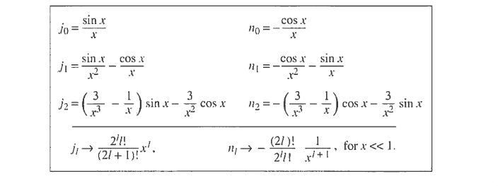
Notice that Bessel functions are finite at the origin, but Neumann functions blow up at the origin. Accordingly, we must have \(B_l = 0\), and hence
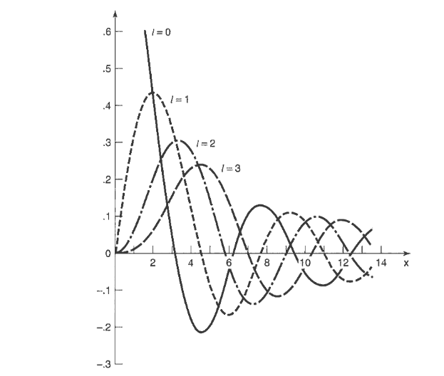
\[ R(r) = Aj_l(kr). \tag{6.47}\]
There remains the boundary condition, \(R(a) = 0\). Evidently \(k\) must be chosen such that
\[ j_l(ka) = 0; \tag{6.48}\]
that is, \((ka)\) is a zero of the \(l\)th-order spherical Bessel function. Let \(\beta_{nl}\) be the \(n\)th zero of \(j_l\). Then
\[ k = \frac{1}{a}\beta_{nl}. \tag{6.49}\]
The allowed energies are given by
\[ E_{nl} = \frac{\hbar^2}{2ma^2}\beta_{nl}^2, \tag{6.50}\]
and the wave functions are
\[ \psi_{nlm}(r,\theta,\phi) = A_{nl}\,j_l(\beta_{nl}r/a)\,Y_l^m(\theta,\phi), \tag{6.51}\]
with the constant \(A_{nl}\) to be determined by normalization. Each energy level is \((2l+1)\)-fold degenerate, since there are \((2l+1)\) different values of \(m\) for each value of \(l\).
6.2 Problems
(a) From the definition (Eq. 6.46), construct \(n_1(x)\) and \(n_2(x)\).
(b) Expand the sines and cosines to obtain approximate formulas for \(n_1(x)\) and \(n_2(x)\), valid when \(x\ll 1\). Confirm that they blow up at the origin.
(a) Check that \(Arj_1(kr)\) satisfies the radial equation with \(V=0\) and \(l=1\).
(b) Determine graphically the allowed energies for the infinite spherical well, when \(l=1\). Show that for large \(n\), \(E_{n1} \approx (\hbar^2\pi^2/2ma^2)(n+1/2)^2\). Hint: First show that \(j_1(x)=0 \Rightarrow x = \tan x\). Plot \(x\) and \(\tan x\) on the same graph, and locate the points of intersection.
A particle of mass \(m\) is placed in a finite spherical well:
\[ V(r) = \begin{cases} -V_0, & \text{if } r\leq a;\\ 0, & \text{if } r>a. \end{cases} \]
Find the ground state, by solving the radial equation with \(l=0\). Show that there is no bound state if \(V_0 a^2 < \pi^2\hbar^2/8m\).
6.3 The Hydrogen Atom
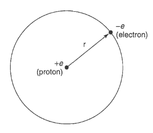
The hydrogen atom consists of a heavy, essentially motionless proton (we may as well put it at the origin), of charge \(e\), together with a much lighter electron (charge \(-e\)) that orbits around it, bound by the mutual attraction of opposite charges (see Fig. 6.3). From Coulomb’s law, the potential energy (in SI units) is
\[ V(r) = -\frac{e^2}{4\pi\epsilon_0}\frac{1}{r}. \tag{6.52}\]
and the radial equation (Eq. 6.37) says
\[ -\frac{\hbar^2}{2m}\frac{d^2u}{dr^2} + \left[-\frac{e^2}{4\pi\epsilon_0}\frac{1}{r} + \frac{\hbar^2}{2m}\frac{l(l+1)}{r^2}\right]u = Eu. \tag{6.53}\]
Our problem is to solve this equation for \(u(r)\), and determine the allowed energies \(E\). The hydrogen atom is such an important case that I’m not going to hand you the solutions this time — we’ll work them out in detail, by the method we used in the analytical solution to the harmonic oscillator.
6.3.1 The Radial Wave Function
Our first task is to tidy up the notation. Let
\[ \kappa \equiv \frac{\sqrt{-2mE}}{\hbar}. \tag{6.54}\]
(For bound states, \(E\) is negative, so \(\kappa\) is real.) Dividing Eq. 6.53 by \(E\), we have
\[ \frac{1}{\kappa^2}\frac{d^2u}{dr^2} = \left[1 - \frac{me^2}{2\pi\epsilon_0\hbar^2\kappa}\frac{1}{(\kappa r)} + \frac{l(l+1)}{(\kappa r)^2}\right]u. \]
This suggests that we introduce
\[ \rho \equiv \kappa r, \qquad\text{and}\qquad \rho_0 \equiv \frac{me^2}{2\pi\epsilon_0\hbar^2\kappa}, \tag{6.55}\]
so that
\[ \frac{d^2u}{d\rho^2} = \left[1 - \frac{\rho_0}{\rho} + \frac{l(l+1)}{\rho^2}\right]u. \tag{6.56}\]
Asymptotic Behaviour
Next we examine the asymptotic form of the solutions. As \(\rho\to\infty\), the constant term dominates, so (approximately)
\[ \frac{d^2u}{d\rho^2} = u. \]
The general solution is
\[ u(\rho) = Ae^{-\rho} + Be^{\rho}, \tag{6.57}\]
but \(e^\rho\) blows up (as \(\rho\to\infty\)), so \(B=0\). Evidently,
\[ u(\rho) \sim Ae^{-\rho}, \tag{6.58}\]
for large \(\rho\). On the other hand, as \(\rho\to 0\) the centrifugal term dominates; approximately, then:
\[ \frac{d^2u}{d\rho^2} = \frac{l(l+1)}{\rho^2}u. \]
The general solution is \(u(\rho) = C\rho^{l+1} + D\rho^{-l}\), but \(\rho^{-l}\) blows up (as \(\rho\to 0\)), so \(D=0\). Thus
\[ u(\rho) \sim C\rho^{l+1}, \tag{6.59}\]
for small \(\rho\).
Peeling Off the Asymptotics
The next step is to peel off the asymptotic behavior, introducing the new function \(v(\rho)\):
\[ u(\rho) = \rho^{l+1}e^{-\rho}v(\rho), \tag{6.60}\] in the hope that \(v(\rho)\) will turn out to be simpler than \(u(\rho)\). The first indications are not auspicious:
\[ \frac{du}{d\rho} = \rho^l e^{-\rho} \left[ (l+1-\rho)v + \rho \frac{dv}{d\rho} \right]. \]
and
\[ \begin{aligned} \frac{d^2u}{d\rho^2} = \rho^l e^{-\rho} \Bigg\{ & \left[ -2l-2+\rho+\frac{l(l+1)}{\rho} \right]v \\[6pt] &+ 2(l+1-\rho)\frac{dv}{d\rho} + \rho\frac{d^2v}{d\rho^2} \Bigg\}. \end{aligned} \]
In terms of \(v(\rho)\), then, the radial equation (Eq. 6.56) reads
\[ \rho\frac{d^2v}{d\rho^2} + 2(l+1-\rho)\frac{dv}{d\rho} + [\rho-2(l+1)]v = 0. \tag{6.61}\]
Power Series Solution
Finally, we assume the solution \(v(\rho)\) can be expressed as a power series in \(\rho\):
\[ v(\rho) = \sum_{j=0}^{\infty}c_j\rho^j. \tag{6.62}\]
Our problem is to determine the coefficients \((c_0, c_1, c_2, \ldots)\). Differentiating term by term:
\[ \frac{dv}{d\rho} = \sum_{j=0}^{\infty}jc_j\rho^{j-1} = \sum_{j=0}^{\infty}(j+1)c_{j+1}\rho^j. \]
\[ \frac{d^2v}{d\rho^2} = \sum_{j=0}^{\infty}j(j+1)c_{j+1}\rho^{j-1}. \]
Inserting these into Eq. 6.61 and equating the coefficients of like powers yield the recursion formula:
\[ \boxed{c_{j+1} = \left\{\frac{2(j+l+1)-\rho_0}{(j+1)(j+2l+2)}\right\}c_j.} \tag{6.63}\]
This recursion formula determines the coefficients, and hence the function \(v(\rho)\): We start with \(c_0\) (this becomes an overall constant, to be fixed eventually by normalization), and Eq. 6.63 gives us \(c_1\); putting this back in, we obtain \(c_2\), and so on.
Termination Condition and Energy Quantization
Now let’s see what the coefficients look like for large \(j\). In this regime the recursion formula says
\[ c_{j+1} \cong \frac{2j}{j(j+1)}c_j = \frac{2}{j+1}c_j. \]
Suppose this were exact. Then \(c_j = 2^j/j!\,c_0\), so
\[ v(\rho) = c_0\sum_{j=0}^{\infty}\frac{2^j}{j!}\rho^j = c_0 e^{2\rho}, \]
and hence \(u(\rho) = c_0\rho^{l+1}e^{\rho}\), which blows up at large \(\rho\). There is only one way out of this dilemma: The series must terminate. There must occur some maximal integer \(j_{\max}\), such that
\[ c_{(j_{\max}+1)} = 0, \tag{6.64}\]
(and beyond which all coefficients vanish automatically). Evidently (Eq. 6.63)
\[ 2(j_{\max}+l+1)-\rho_0 = 0. \]
Defining
\[ n \equiv j_{\max} + l + 1 \tag{6.65}\]
(the so-called principal quantum number), we have
\[ \rho_0 = 2n. \tag{6.66}\]
But \(\rho_0\) determines \(E\) (Eq. 6.54 and Eq. 6.55):
\[ E = -\frac{\hbar^2\kappa^2}{2m} = -\frac{me^4}{8\pi^2\epsilon_0^2\hbar^2\rho_0^2}, \]
so the allowed energies are
\[ \boxed{E_n = -\left[\frac{m}{2\hbar^2}\left(\frac{e^2}{4\pi\epsilon_0}\right)^2\right]\frac{1}{n^2} = \frac{E_1}{n^2}, \quad n=1,2,3,\ldots} \tag{6.67}\]
This is the famous Bohr formula — by any measure the most important result in all of quantum mechanics. Bohr obtained it in 1913 by a serendipitous mixture of inapplicable classical physics and premature quantum theory (the Schrödinger equation did not come until 1924).
Combining Eq. 6.55 and Eq. 6.66, we find that
\[ \kappa = \left(\frac{me^2}{4\pi\epsilon_0\hbar^2}\right)\frac{1}{n} = \frac{1}{an}, \tag{6.68}\]
where
\[ \boxed{a \equiv \frac{4\pi\epsilon_0\hbar^2}{me^2} = 0.529\times 10^{-10}\ \text{m}} \tag{6.69}\]
is the so-called Bohr radius. It follows (again, from Eq. 6.55) that
\[ \rho = \frac{r}{an}. \tag{6.70}\]
The spatial wave functions for hydrogen are labeled by three quantum numbers (\(n\), \(l\), and \(m\)):
\[ \psi_{nlm}(r,\theta,\phi) = R_{nl}(r)\,Y_l^m(\theta,\phi), \tag{6.71}\]
where (referring back to Eq. 6.36 and Eq. 6.60)
\[ R_{nl}(r) = \frac{1}{r}\rho^{l+1}e^{-\rho}v(\rho), \tag{6.72}\]
and \(v(\rho)\) is a polynomial of degree \(j_{\max} = n-l-1\) in \(\rho\), whose coefficients are determined (up to an overall normalization factor) by the recursion formula
\[ c_{j+1} = \frac{2(j+l+1-n)}{(j+1)(j+2l+2)}c_j. \tag{6.73}\]
6.3.2 Ground State and Low-Lying States
The ground state (the state of lowest energy) is the case \(n=1\); putting in the accepted values for the physical constants, we get:
\[ \boxed{E_1 = -\left[\frac{m}{2\hbar^2}\left(\frac{e^2}{4\pi\epsilon_0}\right)^2\right] = -13.6\ \text{eV.}} \tag{6.74}\]
Eq. 6.65 forces \(l=0\), whence also \(m=0\), so
\[ \psi_{100}(r,\theta,\phi) = R_{10}(r)\,Y_0^0(\theta,\phi). \tag{6.75}\]
The recursion formula truncates after the first term (\(j=0\) yields \(c_1=0\)), so \(v(\rho)\) is a constant (\(c_0\)), and
\[ R_{10}(r) = \frac{c_0}{a}e^{-r/a}. \tag{6.76}\]
Normalizing it:
\[ \int_0^\infty|R_{10}|^2 r^2\,dr = \frac{|c_0|^2}{a^2}\int_0^\infty e^{-2r/a}r^2\,dr = |c_0|^2\frac{a}{4} = 1, \]
so \(c_0 = 2/\sqrt{a}\). Meanwhile, \(Y_0^0 = 1/\sqrt{4\pi}\), and hence the ground state of hydrogen is
\[ \boxed{\psi_{100}(r,\theta,\phi) = \frac{1}{\sqrt{\pi a^3}}e^{-r/a}.} \tag{6.77}\]
If \(n=2\) the energy is
\[ E_2 = \frac{-13.6\ \text{eV}}{4} = -3.4\ \text{eV}; \tag{6.78}\]
this is the first excited state — or rather, states, since we can have either \(l=0\) (in which case \(m=0\)) or \(l=1\) (with \(m=-1,0,\) or \(+1\)); evidently four different states share this same energy. If \(l=0\), the recursion relation (Eq. 6.73) gives
\[ c_1 = -c_0 \quad (\text{using }j=0), \qquad\text{and}\qquad c_2 = 0 \quad (\text{using }j=1), \]
so \(v(\rho) = c_0(1-\rho)\), and therefore
\[ R_{20}(r) = \frac{c_0}{2a}\!\left(1 - \frac{r}{2a}\right)e^{-r/2a}. \tag{6.79}\]
If \(l=1\) the recursion formula terminates the series after a single term; \(v(\rho)\) is a constant, and we find
\[ R_{21}(r) = \frac{c_0}{4a^2}r\,e^{-r/2a}. \tag{6.80}\]
(In each case the constant \(c_0\) is to be determined by normalization — see Problem 4.11.)
For arbitrary \(n\), the possible values of \(l\) (consistent with Eq. 6.65) are
\[ l = 0,\,1,\,2,\,\ldots,\,n-1, \tag{6.81}\]
and for each \(l\) there are \((2l+1)\) possible values of \(m\) (Eq. 6.29), so the total degeneracy of the energy level \(E_n\) is
\[ d(n) = \sum_{l=0}^{n-1}(2l+1) = n^2. \tag{6.82}\]
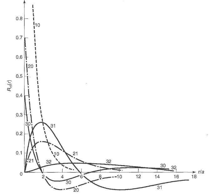
The first few radial wave functions \(R_{nl}(r)\) are plotted in Fig. 6.4.
The polynomial \(v(\rho)\) (defined by the recursion formula, Eq. 6.73) is a function well known to applied mathematicians; apart from normalization, it can be written as
\[ v(\rho) = L_{n-l-1}^{2l+1}(2\rho), \tag{6.83}\]
where
\[ L_{q-p}^p(x) \equiv (-1)^p\!\left(\frac{d}{dx}\right)^{\!p}L_q(x) \tag{6.84}\]
is an associated Laguerre polynomial, and
\[ L_q(x) \equiv e^x\!\left(\frac{d}{dx}\right)^{\!q}(e^{-x}x^q) \tag{6.85}\]
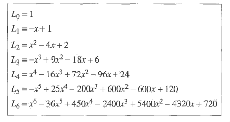
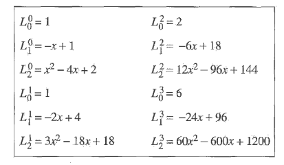
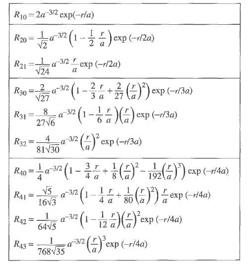
is the \(q\)th Laguerre polynomial. (The first few Laguerre polynomials are listed in Table 6.5; some associated Laguerre polynomials are given in Table 6.6. The first few radial wave functions are listed in Table 6.7, and plotted in Fig. 6.4.)
The normalized hydrogen wave functions are \[ \boxed{ \begin{aligned} \psi_{nlm} = & \sqrt{ \left(\frac{2}{na}\right)^3 \frac{(n-l-1)!}{2n[(n+l)!]^3} } \,e^{-r/na} \left(\frac{2r}{na}\right)^l \\[6pt] & \times \left[ L_{n-l-1}^{2l+1} \left(\frac{2r}{na}\right) \right] Y_l^m(\theta,\phi). \end{aligned} } \tag{6.86}\]
They are not pretty, but don’t complain — this is one of the very few realistic systems that can be solved at all, in exact closed form. Notice that whereas the wave functions depend on all three quantum numbers, the energies (Eq. 6.67) are determined by \(n\) alone. This is a peculiarity of the Coulomb potential; in the case of the spherical well, you may recall, the energies depend also on \(l\) (Eq. 6.50). The wave functions are mutually orthogonal:
\[ \int\psi_{nlm}^*\,\psi_{n'l'm'}\,r^2\sin\theta\,dr\,d\theta\,d\phi = \delta_{nn'}\delta_{ll'}\delta_{mm'}. \tag{6.87}\] This follows from the orthogonality of the spherical harmonics (Eq. 6.33) and (for \(n \neq n'\)) from the fact that they are eigenfunctions of \(H\) with distinct eigenvalues.
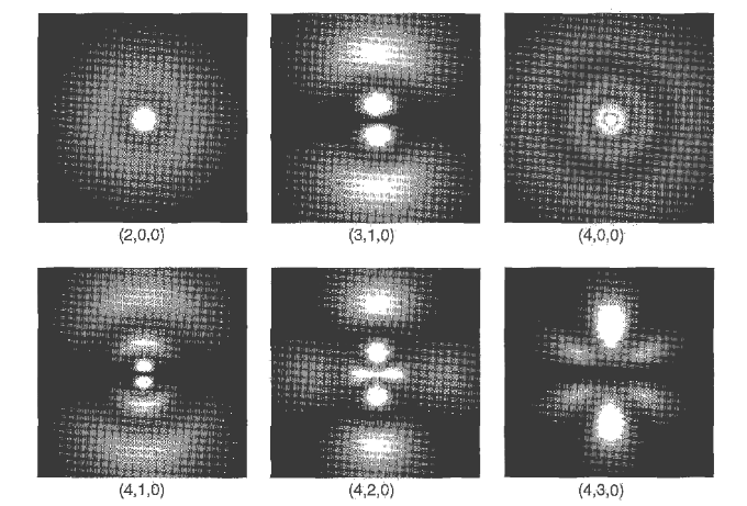
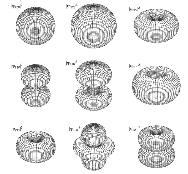
Visualizing the hydrogen wave functions is not easy. Chemists like to draw “density plots,” in which the brightness of the cloud is proportional to \(|\psi|^2\) (Fig. 6.5). More quantitative (but perhaps harder to read) are surfaces of constant probability density (Fig. 6.6).
6.4 Problems
Work out the radial wave functions \(R_{30}\), \(R_{31}\), and \(R_{32}\), using the recursion formula (Eq. 6.73). Don’t bother to normalize them.
(a) Find \(\langle r\rangle\) and \(\langle r^2\rangle\) for an electron in the ground state of hydrogen. Express your answers in terms of the Bohr radius.
(b) Find \(\langle x\rangle\) and \(\langle x^2\rangle\) for an electron in the ground state of hydrogen. Hint: This requires no new integration — note that \(r^2 = x^2+y^2+z^2\), and exploit the symmetry of the ground state.
(c) Find \(\langle x^2\rangle\) in the state \(n=2\), \(l=1\), \(m=1\). Warning: This state is not symmetrical in \(x\), \(y\), \(z\). Use \(x = r\sin\theta\cos\phi\).
What is the most probable value of \(r\), in the ground state of hydrogen? (The answer is not zero!) Hint: First you must figure out the probability that the electron would be found between \(r\) and \(r+dr\).
A hydrogen atom starts out in the following linear combination of the stationary states \(n=2\), \(l=1\), \(m=1\) and \(n=2\), \(l=1\), \(m=-1\):
\[ \Psi(\mathbf{r},0) = \frac{1}{\sqrt{2}}(\psi_{211}+\psi_{21-1}). \]
(a) Construct \(\Psi(\mathbf{r},t)\). Simplify it as much as you can.
(b) Find the expectation value of the potential energy, \(\langle V\rangle\). (Does it depend on \(t\)?) Give both the formula and the actual number, in electron volts.
6.5 The Spectrum of Hydrogen
In principle, if you put a hydrogen atom into some stationary state \(\Psi_{nlm}\), it should stay there forever. However, if you tickle it slightly (by collision with another atom, say, or by shining light on it), the electron may undergo a transition to some other stationary state — either by absorbing energy, and moving up to a higher-energy state, or by giving off energy (typically in the form of electromagnetic radiation), and moving down.
| Series | \(n_f\) | Region |
|---|---|---|
| Lyman | 1 | ultraviolet |
| Balmer | 2 | visible |
| Paschen | 3 | infrared |
| Brackett | 4 | infrared |
Although the wave functions depend on all three quantum numbers \(n\), \(l\), and \(m\), the energies of hydrogen are determined by \(n\) alone. This remarkable degeneracy — \(n^2\) states all sharing the same energy — is a peculiarity of the Coulomb (\(1/r\)) potential.