13 Methods of Electronic Structure Calculations II
13.1 Introduction
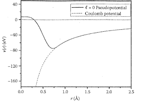
In Chapter Section 12.1, we introduced the concept of pseudopotential, which has emerged as a powerful tool for calculating the electronic structure of solids. A pseudopotential is a weak potential that gives the same eigenvalues as obtained by using the real potential as shown in Fig. 13.1, which shows \(\ell = 0\) pseudopotential and the Coulomb potential for silicon (here, \(\ell\) denotes angular momentum quantum number). One can see that while the Coulomb potential is very strong and approaches infinity near the origin, the pseudopotential is close to zero.
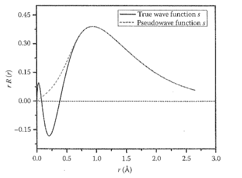
As mentioned in Chapter Section 12.1, the pseudowave function is a very smooth function as compared to the true wave function as shown in Fig. 13.2, which shows the 3s wave function and the pseudowave function for silicon. Because of its smoothness, the pseudowave function requires a smaller number of plane waves in its expansion than needed for the true wave function, thus saving considerable computing costs. In the pseudopotential method, the core electrons are eliminated and one focuses on the valence electrons. In other words, it is assumed that all core levels remain fully occupied and unchanged in all atomic environments. This is known as the frozen core approximation and can be justified because the core electrons are hardly affected by changing the atomic environment. In solid state, the core electrons hardly take any part in properties like bonding or transport. Thus, one can focus only on the valence electrons, reducing the number of electrons in a band structure calculation. The error introduced by such an approximation is quite small but savings in the computational cost is enormous.
Although the idea of pseudopotential was very appealing, its construction posed challenging problems. Since the construction of the pseudopotential method by Phillips and Kleinman (1959) was complicated, initially in the sixties, empirical pseudopotentials were used, which had adjustable parameters obtained by fitting to some experimental results. Since then, the field has made huge progress and now one mostly uses the first-principles pseudopotentials, which have no adjustable parameters and yield results that are in good agreement with the full potential electronic structure calculations. The great advantage of the pseudopotential approach is that it is very efficient and saves a lot of computing cost. Therefore, in this chapter, we shall focus on this method. In Section Section 13.2, we shall take a scattering approach to understand the concept of pseudopotential, which will lead us to the basic principle for constructing an atomic pseudopotential. In Section Section 13.3, we shall briefly discuss how a first-principles atomic pseudopotential is constructed. In Section Section 13.4, we shall derive the secular equation to obtain energy eigenvalues. In Section Section 13.5, we shall discuss the calculation of the total energy. In Section Section 13.6, we very briefly discuss the ultrasoft pseudopotential and PAW methods. In Section Section 13.7, we shall discuss issues regarding the choice of energy cutoff and number of \(k\)-points. In Section Section 13.8, we shall discuss how to handle nonperiodic systems using supercell geometry.
13.2 Scattering Approach to Pseudopotential
In this section, we shall try to understand the concept of pseudopotential using the scattering theory. Let us consider a single muffin-tin potential \(v(r)\), which is defined as
\[ \begin{aligned} v(\vec r) &= v(r) \qquad r \le r_m \\ &= 0 \qquad r \ge r_m \end{aligned} \tag{13.1}\]
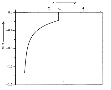
where \(r_m\) is the muffin-tin radius, that is, the muffin-tin potential is spherically symmetric and has a value \(v(r)\) within a sphere of radius \(r_m\) and zero outside the sphere. It is assumed to be attractive and is shown schematically in Fig. 13.3.
An electron moving in this potential will satisfy the Schrödinger equation
\[ \left[-\frac{\hbar^2}{2m_e}\nabla^2+v(\vec r)\right]\psi(\vec r)=\varepsilon\psi(\vec r) \tag{13.2}\]
Since the potential \(v(r)\) is spherically symmetric, the general solution of Eq. 13.2 can be written as
\[ \psi(\vec r)=\sum_L a_L R_l(r)Y_L(\hat r) \tag{13.3}\]
where \(Y_L(\hat r)\) is a spherical harmonic, \(a_L\) expansion coefficient and as before, \(L\) is a composite angular momentum index for \((\ell,m)\). \(R_l(r)\) is the solution of the radial Schrödinger equation
\[ \left[-\frac{1}{2r}\frac{\hbar^2}{m_e}\frac{d^2}{dr^2}r+\frac{\hbar^2}{2m_e}\frac{\ell(\ell+1)}{r^2}+v(r)\right]R_l(r)=\varepsilon R_l(r) \tag{13.4}\]
The solutions of Eq. 13.4 for energy \(\varepsilon \ge 0\) correspond to the scattering states and for \(\varepsilon < 0\), correspond to the bound states. Let us first consider the scattering case when \(\varepsilon \ge 0\). We see from Eq. 13.1 for \(r \ge r_m\) the potential is zero. Therefore, Eq. 13.4 for \(r \ge r_m\) is the radial Schrödinger equation for free electrons. For \(\varepsilon \ge 0\) and \(r \ge r_m\), two linearly independent solutions of Eq. 13.4 are spherical Bessel and Neumann functions \(j_l(kr)\) and \(n_l(kr)\), where \(\varepsilon=(\hbar^2/2m_e)k^2\) (Merzbacher 1998). Thus, for \(r > r_m\), \(R_l(r)\) is a linear combination of \(j_l\) and \(n_l\). Thus
\[ R_l(r)=\cos\delta_l(\varepsilon)j_l(kr)-\sin\delta_l(\varepsilon)n_l(kr) \qquad \text{for } r>r_m \tag{13.5}\]
where \(\delta_l(\varepsilon)\) are energy-dependent parameters and are called phase-shifts. Inside the muffin-tin radius, \(R_l(r)\) is the solution that is regular at the origin. At \(r=r_m\) its logarithmic derivative
\[ \gamma_l(\varepsilon)=\frac{1}{R_l}\frac{dR_l}{dr}\bigg|_{r=r_m} \tag{13.6}\]
must be equal to the log derivative of \(R_l(r)\) from the outside given by Eq. 13.5. From this condition, we can express phase-shifts \(\delta_l(\varepsilon)\)
\[ \delta_l(\varepsilon)=\cot^{-1}\left[\frac{k n_l'-\gamma_l n_l}{k j_l'-\gamma_l j_l}\right]_{r=r_m} \tag{13.7}\]
where prime denotes the derivative.
Let us now look at the asymptotic form (i.e., \(r \rightarrow \infty\)) of \(R_l(r)\). The asymptotic forms of \(j_l(kr)\) and \(n_l(kr)\) are given by
\[ \lim_{r\to\infty} j_l(kr)=\sin(kr-\ell\pi/2)/kr \tag{13.8}\]
\[ \lim_{r\to\infty} n_l(kr)=-\cos(kr-\ell\pi/2)/kr \tag{13.9}\]
Substituting these in Eq. 13.5, we get the asymptotic form for \(R_l(r)\)
\[ \lim_{r\to\infty} R_l(r)=\frac{1}{kr}\sin(kr-\ell\pi/2+\delta_l(\varepsilon)) \tag{13.10}\]
From Eq. 13.10, we see that the asymptotic form of \(R_l(r)\) differs from Eq. 13.8, the asymptotic form of \(v(r)=0\) regular solution, by a shift of phase \(\delta_l(\varepsilon)\). Thus, \(\delta_l(\varepsilon)\) is called as phase-shift.
For the case, \(\varepsilon<0\), which corresponds to bound states, the solution of Eq. 13.4 for \(v(r)=0\) must decay exponentially for \(r>r_m\). The solution outside \(r_m\) is Hankel function of the first kind (Merzbacher 1998), that is
\[ R_l(r)=Ah_l^{(1)}(kr) \qquad r>r_m \tag{13.11}\]
where \(k=\sqrt{2m_e\varepsilon/\hbar^2}\) is now imaginary.
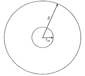
Let us now look at the solution of the free electron (\(v(r)=0\)) problem with spherical boundary condition. We already know the solution of this problem with periodic boundary condition, which gives \(\varepsilon=(\hbar^2/2m_e)k^2\) and \(\psi=Ae^{i\vec k\cdot\vec r}\). Let us solve the same problem with spherical boundary condition. We assume a spherical crystal of large radius \(R\) and take the origin at the center of the sphere. The potential is zero inside the sphere and is infinite outside the sphere. Therefore, the regular solution \(j_l(kR)\) (Eq. 13.8) must vanish at the surface of the sphere. This implies that
\[ kR-\ell\pi/2=n\pi \tag{13.12}\]
where \(n\) is an integer. This gives
\[ k=(n\pi+\ell\pi/2)/R \tag{13.13}\]
and
\[ \varepsilon=\frac{\hbar^2}{2m_e}k^2=\frac{\hbar^2}{2m_e}(n\pi+\ell\pi/2)^2/R^2 \tag{13.14}\]
Now, let us introduce a single attractive muffin-tin potential \(v(r)\) at the center of the spherical crystal of radius \(R\) as shown in Fig. 13.4.
Since the potential is infinite outside the crystal, \(R_l(r)\) must vanish at the surface of the sphere. Using Eq. 13.10, this gives
\[ kR-\ell\pi/2+\delta_l(\varepsilon)=n\pi \tag{13.15}\]
or
\[ k=(n\pi+\ell\pi/2-\delta_l)/R \]
and
\[ \varepsilon=\frac{\hbar^2}{2m_eR^2}(n\pi+\ell\pi/2-\delta_l)^2 \tag{13.16}\]
Eq. 13.16 shows that the energy eigenvalues are determined by the phase-shifts or log derivatives at the muffin-tin radius. It further shows that by introducing a muffin-tin potential at the center of the big sphere, the energy levels get shifted and this shift depends on \(\delta_l\).
If there is no perturbing potential at the center of the spherical crystal, that is, \(v(r)=0\), the phase-shift \(\delta_l=0\). Let us now introduce an attractive perturbing potential and slowly increase its strength. Note that for attractive potential, the phase-shifts are always positive (see, e.g., Roman 1965). As the strength of the potential increases from zero, the phase-shift grows and the solutions get modified. Let us see how it happens for \(s\)-state (\(\ell=0\)) and \(n=1\). For this case, the boundary condition from Eq. 13.15 is
\[ kR+\delta_0(\varepsilon)=\pi \tag{13.17}\]
As the potential increases, the phase-shift \(\delta_0\) increases toward \(\pi\) and the wave number \(k\) approaches zero. At \(\delta_0=\pi\), \(k=0\), which implies \(\varepsilon=0\), that is, we have reached the bottom of the band. As the attractive potential is increased further, corresponding to a phase-shift greater than \(\pi\), \(\varepsilon\) becomes negative and the nature of the state changes abruptly. For \(\varepsilon<0\), we get a bound state that decays exponentially outside the muffin-tin radius. Thus, we can say that at this strength of the potential, when \(\delta_0\) is slightly greater than \(\pi\), a bound state is formed. We can generalize this result by saying that integral multiples of \(\pi\) in the phase-shift correspond to bound states, that is, in general, \(\delta_l\) can be written as
\[ \delta_l=m\pi+\delta_l' \tag{13.18}\]
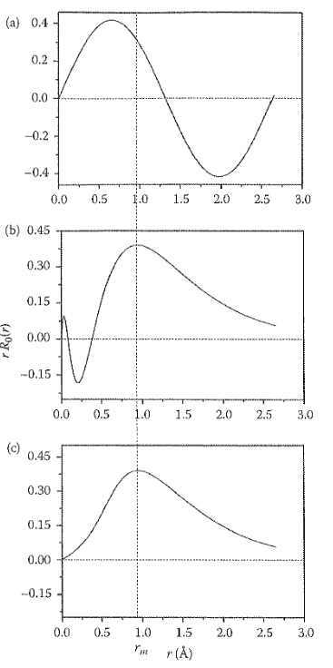
where \(m\) is an integer so that \(\delta_l'\) lies between 0 and \(\pi\). Comparing free electron solution Eq. 13.8 and asymptotic form of \(R_l(r)\) in Eq. 13.10, we see that \(R_l(r)\) will have \(m\) additional nodes. To illustrate this, let us take an example. Assume that \(v(r)\) in Eq. 13.4 corresponds to a Si atom and let us consider 3s wave function, which corresponds to a valence electron. In Fig. 13.5 a, we have plotted \(rR_l(r)\) for a free electron and in Fig. 13.5 b, \(rR_l(r)\) for a 3s valence electron. We see that (i) 3s wave function is phase-shifted compared to the free electron wave function, (ii) it has two nodes (excluding \(r=0\)), that is, \(m=2\) in Eq. 13.18. This is because it has to be orthogonal to 1s (no node) and 2s (1 node) core electron wave functions. This means that \(m\) in Eq. 13.18 also gives a number of core states of angular momentum \(\ell\) below the valence electron state. From the phase-shift point of view, we can understand the oscillations in \(R_l(r)\) as follows. We see that for \(v(r)=0\), there are no bound states and thus no oscillations in the core region. As the potential \(v(r)\) is increased from zero, it pulls more and more of the wave function in the core region, increasing the phase-shift 0 to \(m\pi+\delta_l'\). Whenever the phase-shift increases by \(\pi\), one node is added in the core region. Thus, a stronger attractive potential will give rise to more nodes in the core region.
Let us now bring the pseudopotential into the picture. We know that a pseudopotential is a weak potential that gives the same eigenvalues as the real potential. We also know that pseudopotential is not unique. From the above discussion, it is clear that we may choose a pseudopotential in such a way that it simply eliminates integral multiples of \(\pi\) from the phase-shift (see Eq. 13.18). This will imply that the pseudowave function will have no nodes in the core region (\(r<r_m\)). Also, outside the core region, the pseudowave functions will be equal to the true wave functions. This is illustrated in Fig. 13.5 c, which shows \(rR_l(r)\) for the \(s\) pseudowave function for Si. Thus, the pseudowave function has no rapid oscillations in the core region so that its plane wave expansion is rapidly convergent. Note that such a pseudowave function will give the same logarithmic derivative as the true wave function, as is clear from Eq. 13.7 and Eq. 13.18 and from the fact that \(\cot(m\pi+\delta_l')=\cot\delta_l'\). Thus, the integral multiples of \(\pi\) in Eq. 13.18 have no effect on the log derivatives. Since eigenvalues are determined by the log derivatives, such a pseudopotential, which eliminates integral multiples of \(\pi\) in Eq. 13.18, is guaranteed to give the same eigenvalues as the true potential. This suggests a way of constructing atomic pseudopotentials from first-principles. One first solves the Kohn-Sham equation for an atom and gets the true wave function. Then, one simply removes the nodes of the true wave function in the core region and obtains a pseudowave function. Now, an inverse problem is solved. We try to find a pseudopotential that will give this pseudowave function as its eigenfunction and the true eigenvalues as its eigenvalues. This is the basic principle of constructing first-principles pseudopotentials.
13.3 Construction of First-Principles Atomic Pseudopotentials
As we have discussed earlier, the pseudopotential is not unique. Thus, there is enormous choice in constructing the pseudopotential. As mentioned earlier, empirical pseudopotentials were used in the 1960s, which were determined by fitting experimental data. Such empirical pseudopotentials have several drawbacks, namely
The pseudopotential constructed for one environment of an atom will not work for another environment, that is, they lack transferability.
Although simple to use, they are not obtained from first-principles.
During the last two decades or so, there has been a revolution in the use of first-principles atomic pseudopotentials. All first-principles pseudopotentials are generated from all-electron atomic calculations. The basic principle of generating first-principles pseudopotential has already been discussed in Section Section 13.2. Here, we briefly discuss the main steps to construct pseudopotentials (Hamann et al. 1979, Bachelet et al. 1982):
- First of all, true radial wave function \(R_{nl}(r)\) of the atom is obtained by solving the radial Kohn-Sham equation
\[ \left[-\frac{1}{2r}\frac{\hbar^2}{m_e}\frac{d^2}{dr^2}r+\frac{\hbar^2}{2m_e}\frac{\ell(\ell+1)}{r^2}+v(r)\right]R_{nl}(r)=\varepsilon_{nl}R_{nl}(r) \tag{13.19}\]
where
\[ v(r)=-\frac{e^2}{4\pi\epsilon_0}\frac{Z}{r}+v_H(r)+v_{xc}(r) \tag{13.20}\]
Here, \(v_{xc}(r)\) is the exchange correlation potential and \(v_H(r)\) is given by
\[ v_H(r)=\int\frac{e^2}{4\pi\epsilon_0}\frac{n(r')}{|\vec r-\vec r'|}\,d^3r' \tag{13.21}\]
where \(n(r')\) is the total electron density.
From true radial wave function \(R_{nl}(r)\), a pseudowave function \(\phi_l^{ps}(r)\) is constructed such that it fulfills the following conditions:
The pseudowave function \(\phi_l^{ps}(r)\) should contain no nodes. Since the pseudowave function is constructed only for valence electrons, we omit the principal quantum number \(n\).
The normalized atomic radial pseudowave function \(\phi_l^{ps}(r)\) is equal to normalized radial true wave function \(R_l(r)\) beyond a suitably chosen cutoff radius \(r_c\)
\[ \phi_l^{ps}(r)=R_l(r) \qquad \text{for } r\ge r_c \tag{13.22}\]
The eigenvalues of pseudowave function must be equal to the true eigenvalues.
The charge enclosed within \(r_c\) for the pseudowave function and true wave function must be equal, that is
\[ \int_0^{r_c}|\phi_l^{ps}(r)|^2r^2dr=\int_0^{r_c}|R_l(r)|^2r^2dr \tag{13.23}\]
This is referred to as the norm-conservation condition and if a pseudopotential meets this condition, it is called a “norm-conserving pseudopotential” (NCPP). Note that a pseudowave function fulfilling these conditions can be constructed arbitrarily in many ways. This freedom is further exploited to produce a smooth pseudopotential.
- Once the pseudowave function has been obtained, the radial Schrödinger equation can be inverted to yield a screened pseudopotential that has the pseudowave function as its eigenfunction at the correct eigenvalue.
\[ \left[-\frac{1}{2r}\frac{\hbar^2}{m_e}\frac{d^2(r\phi_l^{ps}(r))}{dr^2}+\frac{\hbar^2}{2m_e}\frac{\ell(\ell+1)}{r^2}\phi_l^{ps}(r)+w_l^{sc}\phi_l^{ps}(r)\right]=\varepsilon_l\phi_l^{ps}(r) \tag{13.24}\]
Eq. 13.24 implies that the pseudowave function must have continuous derivatives up to the second derivative if we want a continuous pseudopotential. Since the true wave function satisfies Eq. 13.24 with true potential \(v(r)\) and since for \(r\ge r_c\), \(\phi_l^{ps}(r)=R_l(r)\), the screened pseudopotential \(w_l^{sc}(r)\) and the true potential are identical beyond \(r_c\).
The screened pseudopotential \(w^{sc}\) thus obtained lacks transferability as the screening from the valence electrons depends strongly on the environment in which they are placed. Thus, the first step to improve transferability is to remove the screening effects of the valence electrons and generate an ionic pseudopotential \(w\). This is done by subtracting \(v_H(r)\) and \(v_{xc}(r)\), calculated by using the valence pseudowave function, from \(w^{sc}\), that is
\[ w_l(r)=w_l^{sc}(r)-v_H(r)-v_{xc}(r) \tag{13.25}\]
where
\[ v_H(r)=\int\frac{e^2}{4\pi\epsilon_0}\frac{n^v(r')}{|\vec r-\vec r'|}\,d^3r' \tag{13.26}\]
and \(v_{xc}(r)\) is also calculated from \(n^v(r)\), where \(n^v(r)\) is the valence electron density.
\[ n^v(r)=\sum_{\ell,\mathrm{occupied}}|\phi_l^{ps}(r)|^2 \tag{13.27}\]
When such an ionic potential is placed in a different environment, \(v_H(r)\) and \(v_{xc}(r)\) are recalculated for that environment and again added to the potential. Note that this does not guarantee that the pseudopotential is transferable to any environment. It can be used only in an environment in which eigenvalues do not change significantly from the eigenvalues used in its construction. The property that makes this energy range wider is loosely called smoothness, that is, the smoother the pseudopotential, the weaker the energy dependence.
In summary, the following conditions for the construction of pseudopotentials should be satisfied:
The pseudowave function \(\phi^{ps}(r)\) is nodeless and is identical to the true wave function outside a suitably chosen cutoff radius \(r_c\).
The first and second derivatives of the pseudowave function are continuous at \(r_c\).
The eigenvalues of the pseudowave functions coincide with those of true wave functions.
The norm of the true and pseudowave functions inside \(r_c\) is the same
\[ \int_0^{r_c}|r\phi^{ps}(r)|^2dr=\int_0^{r_c}|rR_l(r)|^2dr \tag{13.28}\]
- Further conditions may be imposed to enhance the smoothness of the pseudopotential.
We had seen in Chapter Section 12.1 that the pseudopotential in general will be a nonlocal function, that is, it is not a simple multiplicative factor. The above procedure also shows that the pseudopotential is nonlocal, that is, each component of the wave functions will see a different potential. We see that the pseudopotential so generated is local in the radial coordinate but nonlocal in the angular coordinates. This potential can be written as
\[ w=\sum_{\ell=0}^{\infty}\sum_{m=-\ell}^{\ell}|\ell m\rangle w^\ell(r)\langle\ell m| \tag{13.29}\]
\[ =\sum_{\ell}w^\ell(r)\hat P_\ell \tag{13.30}\]
where \(|\ell m\rangle\) are the spherical harmonics and \(\hat P_\ell=\sum_{m=-\ell}^{\ell}|\ell m\rangle\langle\ell m|\) is the projection operator. Here, \(w^\ell(r)\) is the pseudopotential for the angular component \(\ell\). When such a pseudopotential acts on a wave function, it decomposes it into its spherical harmonics components and then each of it is multiplied by the corresponding pseudopotential. Since \(w^\ell(r)\) is a local operator in the radial coordinate, such a potential is called semilocal potential.
The summation on \(\ell\) in Eq. 13.30 is truncated at some value of \(\ell=\ell_{max}\). The pseudopotential then can be written as
\[ w=w_{loc}(r)+\sum_{\ell=0}^{\ell_{max}}w^\ell_{nonlocal}(r)\hat P_\ell \tag{13.31}\]
where
\[ w^\ell_{nonlocal}(r)=w^\ell(r)-w_{loc}(r) \tag{13.32}\]
Here, \(w_{loc}(r)\) is the local part that is normally chosen as the pseudopotential for the first angular momentum that is not represented in the core, for example, \(w^d(r)\) for Si. The idea is that it should represent those angular components of the pseudopotential adequately that are not corrected by the nonlocal part. The nonlocal part \(w^\ell_{nonlocal}(r)\) as defined by Eq. 13.32 is the difference between the \(\ell\)-dependent potential \(w^\ell(r)\) and \(w_{loc}(r)\). Since \(w^\ell(r)\) and \(w_{loc}(r)\) are identical outside the cutoff radius, \(w^\ell_{nonlocal}(r)\) is zero outside the cutoff radius. Thus, \(w^\ell_{nonlocal}(r)\) are short-ranged functions confined to the core region.
Other methods of pseudopotential construction that are quite popular are due to Troullier and Martins and due to Vanderbilt. Smoothest norm-conserving potentials are obtained by using the Troullier and Martins’ construction (1991). On the other hand, Vanderbilt (1990) used a non-norm-conserving pseudopotential to obtain “ultrasoft” pseudopotential (see Section Section 13.6).
13.4 Secular Equation
We shall derive the secular equation for the NCPP. Here, we shall consider a more general case when we have \(M\) identical atoms in a unit cell at positions \(\vec d_j\) and when the pseudopotential is nonlocal. The formulation can be easily generalized to many different types of atoms per unit cell. The total pseudopotential \(W\) can be written as
\[ W(\vec r,\vec r')=\sum_{i,j}w(\vec r-\vec R_i-\vec d_j,\vec r'-\vec R_i-\vec d_j) \tag{13.33}\]
where \(w\) is the atomic pseudopotential and \(\vec R_i\) is a lattice vector. The general Hamiltonian can be written as
\[ H=-\frac{\hbar^2}{2m_e}\nabla^2+v_H(\vec r)+v_{xc}(\vec r)+W \tag{13.34}\]
where \(v_{xc}(\vec r)\) is the exchange correlation potential, \(v_H(\vec r)\) is the Hartree potential given by \(v_H(\vec r)=\int(e^2/4\pi\epsilon_0)n(\vec r')d^3r'/|\vec r-\vec r'|\). Here, \(n(\vec r)\) is the charge density of the valence electrons given by \(n(\vec r)=\sum_k^{occ}|\phi_k^{ps}(\vec r)|^2\). The pseudowave function \(\phi_k^{PS}(\vec r)\) is expanded in plane waves as
\[ \begin{aligned} \phi_k^{PS}(\vec r)&=\frac{1}{\sqrt{\Omega}}\sum_{\vec G}c_{\vec k+\vec G}\exp[i(\vec k+\vec G)\cdot\vec r]\\ &=\sum_{\vec G}c_{\vec k+\vec G}|\vec k+\vec G\rangle \end{aligned} \tag{13.35}\]
We want to solve the equation
\[ H\phi_k^{PS}(\vec r)=\varepsilon_k\phi_k^{PS}(\vec r) \tag{13.36}\]
By multiplying Equation Eq. 13.36 by \(\langle \vec{k}+\vec{G}|\), we get
\[ \left\langle \vec{k}+\vec{G} \left| H \right| \phi_k^{PS}(\vec r) \right\rangle = \varepsilon_k \left\langle \vec{k}+\vec{G} \middle| \phi_k^{PS}(\vec r) \right\rangle \tag{13.37}\]
Substitution of Equation Eq. 13.35 in Equation Eq. 13.37 gives
\[ \sum_{\vec G'} H_{\vec k+\vec G,\vec k+\vec G'} c_{\vec k+\vec G'} = \varepsilon_k c_{\vec k+\vec G} \tag{13.38}\]
where
\[ H_{\vec k+\vec G,\vec k+\vec G'}=\langle\vec k+\vec G|H|\vec k+\vec G'\rangle \tag{13.39}\]
Eq. 13.38 is the secular equation by solving which energies \(\varepsilon_k\) can be found.
Let us now calculate matrix element (Eq. 13.39). The matrix element of kinetic energy operator is very easy to evaluate and is given by
\[ \left\langle\vec k+\vec G\left|-\frac{\hbar^2}{2m_e}\nabla^2\right|\vec k+\vec G'\right\rangle=\frac{\hbar^2}{2m_e}|\vec k+\vec G|^2\delta_{\vec G,\vec G'} \tag{13.40}\]
The Hartree potential is given by
\[ \begin{aligned} v_H(\vec r)&=\int\frac{e^2}{4\pi\epsilon_0}\frac{n(\vec r')d^3r'}{|\vec r-\vec r'|}\\ &=\int d^3r'\frac{e^2}{4\pi\epsilon_0}\sum_{\vec G}n(\vec G)e^{i\vec G\cdot\vec r'}\sum_{\vec q}\frac{4\pi}{q^2}e^{i\vec q\cdot(\vec r-\vec r')}\\ &=\sum_{\vec G,\vec q}n(\vec G)\frac{e^2}{4\pi\epsilon_0}\frac{4\pi}{q^2}e^{i\vec q\cdot\vec r}\delta_{\vec q,\vec G}\\ &=\sum_{\vec G}n(\vec G)\frac{e^2}{4\pi\epsilon_0}\frac{4\pi}{|\vec G|^2}e^{i\vec G\cdot\vec r} \end{aligned} \tag{13.41}\]
where \(n(\vec G)\) is the Fourier transform of the charge density \(n(\vec r)\). Now, the matrix element of \(v_H(\vec r)\) can be written as
\[ \begin{aligned} \langle\vec k+\vec G|v_H(\vec r)|\vec k+\vec G'\rangle&=\frac{1}{\Omega}\int v_H(\vec r)e^{-i(\vec G-\vec G')\cdot\vec r}d^3r=v_H(\vec G-\vec G')\\ &=n(\vec G-\vec G')\frac{e^2}{4\pi\epsilon_0}\frac{4\pi}{|\vec G-\vec G'|^2} \end{aligned} \tag{13.42}\]
The pseudopotential \(W\) can be divided into two parts as
\[ W(\vec r,\vec r')=W^{loc}(\vec r)+W^{nl}(\vec r,\vec r') \tag{13.43}\]
Let us first calculate the matrix element of the local part. We can write it as
\[ \begin{aligned} \langle\vec k+\vec G|W^{loc}|\vec k+\vec G'\rangle&=\frac{1}{\Omega}\int W^{loc}(\vec r)e^{-i(\vec G-\vec G')\cdot\vec r}d^3r\\ &=\frac{1}{\Omega}\int\sum_{i,j}w^{loc}(\vec r-\vec R_i-\vec d_j)e^{-i(\vec G-\vec G')\cdot\vec r}d^3r\\ &=\frac{1}{\Omega}\sum_{i,j}\int w^{loc}(\vec r)e^{-i(\vec G-\vec G')\cdot(\vec r+\vec R_i+\vec d_j)}d^3r\\ &=\frac{N}{\Omega}\sum_j\int w^{loc}(\vec r)e^{-i(\vec G-\vec G')\cdot(\vec r+\vec d_j)}d^3r\\ &=\frac{N}{\Omega}\sum_j e^{-i(\vec G-\vec G')\cdot\vec d_j}\int w^{loc}(\vec r)e^{-i(\vec G-\vec G')\cdot\vec r}d^3r\\ &=S(\vec G-\vec G')w^{loc}(\vec G-\vec G') \end{aligned} \tag{13.44}\]
where \(S(\vec q)\) is the geometrical structure factor given by
\[ S(\vec q)=\sum_j e^{-i\vec q\cdot\vec d_j} \tag{13.45}\]
and \(w^{loc}(\vec G)\) is the Fourier transform of the local atomic pseudopotential given by
\[ w^{loc}(\vec G)=\frac{N}{\Omega}\int w^{loc}(\vec r)e^{-i\vec G\cdot\vec r}d^3r=\frac{1}{\Omega_{cell}}\int w^{loc}(\vec r)e^{-i\vec G\cdot\vec r}d^3r \tag{13.46}\]
where \(\Omega_{cell}=\Omega/N\) is the unit cell volume. Note that the \(\vec G=0\) matrix element of \(v_H(r)\) diverges as \(1/G^2\). The \(\vec G=0\) matrix element of the bare ion-electron Coulomb interaction will also diverge as \(1/G^2\). The local pseudopotential will have the same long-range behavior since at large distances the ion cores will look like point particles. The sum of the two contributions will diverge as \(4\pi Q_T/G^2\), where \(Q_T\) is the total charge in the unit cell. Thus, to avoid \(\vec G=0\) divergence, such calculations can be done only for the charge-neutral systems.
The nonlocal part of the pseudopotential \(W^{nl}\) can be expanded in terms of atomic contributions \(w^{nl}\) as
\[ W^{nl}(\vec r,\vec r')=\sum_{i,j}w^{nl}(\vec r-\vec R_i-\vec d_j,\vec r'-\vec R_i-\vec d_j) \]
Thus
\[ \begin{aligned} \langle\vec k+\vec G|W^{nl}|\vec k+\vec G'\rangle &= \sum_{i,j} \langle \vec k+\vec G | w^{nl}( \vec r-\vec R_i-\vec d_j, \vec r'-\vec R_i-\vec d_j ) | \vec k+\vec G' \rangle \\ &= \frac{1}{\Omega} \iint \sum_{i,j} e^{-i(\vec k+\vec G)\cdot\vec r} w^{nl}( \vec r-\vec R_i-\vec d_j, \vec r'-\vec R_i-\vec d_j ) \\ &\qquad\times e^{i(\vec k+\vec G')\cdot\vec r'} \,d^3r\,d^3r' \\ &= \frac{1}{\Omega} \iint \sum_{i,j} e^{-i(\vec k+\vec G)\cdot (\vec r+\vec R_i+\vec d_j)} w^{nl}(\vec r,\vec r') \\ &\qquad\times e^{i(\vec k+\vec G')\cdot (\vec r'+\vec R_i+\vec d_j)} \,d^3r\,d^3r' \\ &= N \sum_j e^{-i(\vec G-\vec G')\cdot\vec d_j} \langle \vec k+\vec G | w^{nl} | \vec k+\vec G' \rangle \\ &= NS(\vec G-\vec G') \langle \vec k+\vec G | w^{nl} | \vec k+\vec G' \rangle \end{aligned} \tag{13.47}\]
The matrix elements of \(w^{nl}\) can be written as
\[ \begin{aligned} \langle \vec k+\vec G | w^{nl}(\vec r,\vec r') | \vec k+\vec G' \rangle &= \sum_\ell \Biggl\langle \vec k+\vec G \Biggl| w_\ell^{nl}(r) \frac{1}{r^2} \delta(r-r') \\ &\qquad\times \sum_m Y_{\ell m}^{*}(\vec r) Y_{\ell m}(\vec r') \Biggr| \vec k+\vec G' \Biggr\rangle \\ &= \frac{1}{\Omega} \sum_\ell \iint d^3r\,d^3r' \, e^{-i(\vec k+\vec G)\cdot\vec r} w_\ell^{nl}(r) \frac{1}{r^2} \delta(r-r') \\ &\qquad\times Y_{\ell m}^{*}(\vec r) Y_{\ell m}(\vec r') e^{i(\vec k+\vec G')\cdot\vec r'} \end{aligned} \tag{13.48}\]
where we have assumed the pseudopotential to be of semilocal form (Eq. 13.30). Let us evaluate Eq. 13.48 by expanding the plane waves in terms of spherical harmonics with respect to the center of the atom as
\[ e^{+i(\vec k+\vec G')\cdot\vec r'}=4\pi\sum_{\ell=0}^{\infty}\sum_{m=-\ell}^{+\ell}i^\ell j_\ell(|\vec k+\vec G'|r')Y_{\ell m}(\vec k+\vec G')Y_{\ell m}^{*}(\vec r') \]
Substituting this in Eq. 13.48, we get
\[ \begin{aligned} w_{\vec k+\vec G,\vec k+\vec G'}^{nl}&=\frac{1}{\Omega}\sum_\ell\iint r^2drd\Omega\,r'^2dr'd\Omega'\\ &\times(4\pi)^2\sum_{L_1}i^{-\ell_1}j_{\ell_1}(|\vec k+\vec G|r)Y_{L_1}^{*}(\vec k+\vec G)Y_{L_1}(\vec r)\\ &\times w_\ell^{nl}\frac{1}{r^2}\delta(r-r')Y_L^{*}(\vec r)Y_L(\vec r')\\ &\times\sum_{L_2}i^{\ell_2}j_{\ell_2}(|\vec k+\vec G'|r)Y_{L_2}(\vec k+\vec G')Y_{L_2}^{*}(\vec r') \end{aligned} \tag{13.49}\]
where we have used a composite index \(L=(\ell,m)\).
Now, we use the addition theorem for spherical harmonics (see, e.g., Quantum Mechanics by Merzbacher (1998))
\[ P_\ell(\cos\theta_{\vec k+\vec G,\vec k+\vec G'})=\frac{4\pi}{2\ell+1}\sum_{m=-\ell}^{+\ell}Y_L^{*}(\vec k+\vec G)Y_L(\vec k+\vec G') \tag{13.50}\]
and
\[ \int Y_{L_1}^{*}(\vec r)Y_L(\vec r)d\Omega=\delta_{L_1L} \tag{13.51}\]
Substitution of Eq. 13.50 and Eq. 13.51 in Eq. 13.49 gives
\[ \begin{aligned} w_{\vec k+\vec G,\vec k+\vec G'}^{nl} &= \frac{1}{\Omega} \sum_\ell 4\pi(2\ell+1) P_\ell( \cos\theta_{\vec k+\vec G,\vec k+\vec G'} ) \\ &\qquad\times \int r^2dr\, j_\ell(|\vec k+\vec G|r) w_\ell^{nl}(r) j_\ell(|\vec k+\vec G'|r) \end{aligned} \tag{13.52}\]
This form of the nonlocal pseudopotential is inconvenient for some applications. Therefore, Kleinman and Bylander (1982) proposed a form that is computationally more efficient. However, we shall not discuss it here and refer to the original paper. The exchange correlation potential is local in space. Thus
\[ \langle\vec k+\vec G|v_{xc}(\vec r)|\vec k+\vec G'\rangle=v_{xc}(\vec G-\vec G') \]
Once all the matrix elements of \(H\) are known, \(\varepsilon_k\) can be calculated from Eq. 13.38.
13.5 Calculation of the Total Energy
The total energy of a solid is a very important quantity, as a large number of its properties can be related to the total energy. For example, the structure and equilibrium lattice constant of the solid could be obtained by optimizing the total energy. Similarly, the bulk moduli can be related to the total energy. Thus, an accurate calculation of the total energy can predict several properties of solids. It is interesting to note that Wigner and Seitz (1955) had commented in 1955 that nothing much would be gained from such a calculation. However, the experience of the last three decades tells a different story. The calculation of the total energy now plays a central role in predicting unknown structures, designing new materials, ab initio molecular dynamics, calculations of phonon spectra, and so on as we shall see in subsequent chapters.
We shall now discuss how the total energy can be calculated using norm-conserving pseudopotentials. In the pseudopotential approximation, the core electrons are frozen and one only needs to calculate the wave functions and energy eigenvalues of the valence electrons. Since the core electrons do not play any role in bonding, this is a very good approximation. Also, it should be noted that in this approximation, the pseudowave function and the true wave function are identical outside the ionic cores. Thus, the total energy \(E\) can be written as
\[ E=E_{kin}+E_{xc}+E_H+E_{ps}^{loc}+E_{ps}^{nl}+V_{II} \tag{13.53}\]
where \(E_{kin}\) is the kinetic energy, \(E_{xc}\) is the exchange correlation energy, \(E_{ps}^{loc}\) and \(E_{ps}^{nl}\) are local and nonlocal pseudopotential energies, respectively, and \(V_{II}\) is the ion-ion repulsive energy.
The kinetic energy of the electrons, \(E_{kin}\), can be written as
\[ \begin{aligned} E_{kin}&=\sum_k\int\phi_k^{*}(\vec r)\left(-\frac{\hbar^2}{2m_e}\nabla^2\right)\phi_k(\vec r)d^3r\\ &=\sum_{\vec k,\vec G}\frac{\hbar^2}{2m_e}(\vec k+\vec G)^2c^{*}(\vec k+\vec G)c(\vec k+\vec G) \end{aligned} \tag{13.54}\]
where \(\phi_k\) is the pseudowave function and for simplicity superscript “PS” over \(\phi_k\) has been dropped. The exchange-correlation energy \(E_{xc}\) is generally calculated in real space. In LDA, it can be calculated using
\[ E_{xc}=\int\varepsilon_{xc}(n(\vec r))n(\vec r)d^3r \tag{13.55}\]
where \(\varepsilon_{xc}\) is obtained from homogeneous electron gas calculation.
The Hartree energy \(E_H\) is given by
\[ \begin{aligned} E_H&=\frac{1}{2}\iint\frac{e^2}{4\pi\epsilon_0}\frac{n(\vec r)n(\vec r')}{|\vec r-\vec r'|}d^3r d^3r'\\ &=\frac{1}{2}\iint\sum_{\vec q}\frac{e^2}{4\pi\epsilon_0}\frac{4\pi}{q^2}e^{i\vec q\cdot(\vec r-\vec r')}\sum_{\vec G\vec G'}n(\vec G)e^{i\vec G\cdot\vec r}n(\vec G')e^{i\vec G'\cdot\vec r'}d^3r d^3r'\\ &=\frac{1}{2}\iint\sum_{\vec q}\sum_{\vec G\vec G'}\frac{e^2}{4\pi\epsilon_0}\frac{4\pi}{q^2}\delta_{\vec q,-\vec G}\delta_{\vec q,\vec G'}n(\vec G)n(\vec G')\\ &=\frac{1}{2}\sum_{\vec G}\frac{e^2}{\epsilon_0}\frac{1}{G^2}n(\vec G)n(-\vec G) \end{aligned} \tag{13.56}\]
where \(n(\vec G)\) is the Fourier transform of \(n(\vec r)\).
\(E_{ps}^{loc}\) in Eq. 13.53 denotes the local pseudopotential energy given by
\[ E_{ps}^{loc}=\int W^{loc}(\vec r)n(\vec r)d^3r \tag{13.57}\]
where \(W^{loc}(\vec r)\) is the local part of the pseudopotential.
\(E_{ps}^{loc}\) can be evaluated as
\[ \begin{aligned} E_{ps}^{loc}&=\sum_k\int\phi_k^{*}(\vec r)W^{loc}(\vec r)\phi_k(\vec r)d^3r\\ &=\sum_{\vec k,\vec G,\vec G'}c^{*}(\vec k+\vec G)\langle\vec k+\vec G|W^{loc}(\vec r)|\vec k+\vec G'\rangle c(\vec k+\vec G')\\ &=\sum_{\vec k,\vec G,\vec G'}c^{*}(\vec k+\vec G)S(\vec G-\vec G')w^{loc}(\vec G-\vec G')c(\vec k+\vec G') \end{aligned} \tag{13.58}\]
\(E_{ps}^{nl}\) is the nonlocal pseudopotential energy given by
\[ E_{ps}^{nl}=\sum_k\int\phi_k^{*}(\vec r)W^{nl}(\vec r,\vec r')\phi_k(\vec r')d^3r d^3r' \tag{13.59}\]
\[ \begin{aligned} E_{ps}^{nl}&=\sum_{\vec k,\vec G,\vec G'}c^{*}(\vec k+\vec G)\langle\vec k+\vec G|W^{nl}(\vec r,\vec r')|\vec k+\vec G'\rangle c(\vec k+\vec G')\\ &=\sum_{\vec k,\vec G,\vec G'}NS(\vec G-\vec G')\langle\vec k+\vec G|w^{nl}|\vec k+\vec G'\rangle c^{*}(\vec k+\vec G)c(\vec k+\vec G') \end{aligned} \tag{13.60}\]
where we have used Eq. 13.48. As we have already calculated \(\langle\vec k+\vec G|w^{nl}|\vec k+\vec G'\rangle\) in Eq. 13.52, \(E_{ps}^{nl}\) can be evaluated.
\(V_{II}\) in Eq. 13.53 is the contribution coming from ion-ion repulsion and is given by
\[ V_{II}=\frac{1}{2}\sum_{\substack{I,J,j\\I\ne j}}\frac{e^2}{4\pi\epsilon_0}\frac{Z_IZ_J}{|\vec R_i+\vec d_i-\vec d_j|} \tag{13.61}\]
The evaluation of \(E_H\), \(E_{ps}^{loc}\), and \(V_{II}\) requires some care in computation because of the long-range nature of these interactions. For evaluating the lattice sum in Eq. 13.58, Ewald’s method is used. For details, we refer to the article by Bagno et al. (1991).
13.6 Ultrasoft Pseudopotential and Projector-Augmented Wave Method
It turns out that the norm-conserving potentials need a large number of plane waves or large energy cutoff (see the next section) for elements with strongly localized orbitals such as transition metal and rare-earth elements, thus requiring much more computational effort. Vanderbilt (1990) showed that this problem could be solved by relaxing the norm-conservation requirement. This greatly reduced the energy cutoff because a large value of \(r_c\) could be used. However, this comes at a price. Since the norm of the pseudowave function is not conserved, it results in the charge deficit. To compensate for this deficit, augmentation charges, which are defined as the charge density difference between true and pseudowave functions, are introduced in the core region. The core radius \(r_c\) can now be chosen quite large, about half the nearest-neighbor distance, making the pseudopotential ultrasoft. Using this method, one can obtain a pseudowave function as smooth as possible in the core region and reduce the number of plane waves needed in the plane wave expansion. The norm-conservation is taken into account afterward by solving a generalized eigenvalue equation. Vanderbilt’s approach works really well for 3-d transition metals. It not only saves computational time but also improves accuracy. Thus, the ultrasoft pseudopotential (US-PP) method has been one of the important developments in the electronic structure methods.
Another very important development is due to Blöchl (1994), who developed the PAW method. The PAW method combines the ideas of the LAPW (see the next chapter) and ultrasoft pseudopotential methods, somewhat similar to the OPW method, which combines the plane wave and tight-binding methods. In this method, the all-electron wave function is decomposed in terms of a smooth pseudowave function and a rapidly varying contribution localized within the core region. The all-electron wave function \(\psi^n_{AE}\), where \(n\) is a composite index for the band, \(\vec k\), and spin, is related to the pseudowave function \(\psi^n_{PS}\) by a linear transformation
\[ |\psi^n_{AE}\rangle=T|\psi^n_{PS}\rangle \tag{13.62}\]
The KS equation can be written as
\[ H|\psi^n_{AE}\rangle=\varepsilon_n|\psi^n_{AE}\rangle \]
\[ HT|\psi^n_{PS}\rangle=\varepsilon_nT|\psi^n_{PS}\rangle \]
or
\[ T^{\dagger}HT|\psi^n_{PS}\rangle=T^{\dagger}T\varepsilon_n|\psi^n_{PS}\rangle \tag{13.63}\]
Pseudowave functions are obtained by solving Eq. 13.63 and then transformed back to true wave functions using Eq. 13.62, which are then used to calculate the charge density and the total energy. Thus, the PAW method is an all-electron method and not a traditional pseudopotential method. It uses frozen core approximation but, in principle, it is not necessary. However, the method is cast in such a way that the machinery of the pseudopotential can be used with slight modification and some additional routines. The PAW method is one of the most powerful and accurate methods with the efficiency of the pseudopotential methods. For details, we refer to the original paper (Blöchl 1994).
13.7 Energy Cutoff and \(k\)-Point Convergence
There are two very important issues that must be settled before doing an electronic structure calculation:
How many plane waves must one use for the expansion of the wave function?
How many \(k\)-points must one use for an accurate determination of the total energy?
In principle, an infinite number of plane waves are required in the plane wave expansions of \(\phi_k^{PS}(\vec r)\) in Eq. 13.34. In practice, the series is terminated at some \(G_{max}\) corresponding to the cutoff energy \(E_{cut}=(\hbar^2/2m_e)G_{max}^2\). A smoother and weaker pseudopotential will require a lower-energy cutoff. The truncation of the series will lead to an error in the calculated quantities, but this can be decreased by increasing energy cutoff. Therefore, it is important to vary \(E_{cut}\) and examine how the total energy converges. The energy cutoff should be chosen such that one gets the total energy close to the converged value.
For Brillouin zone integration, one uses a discrete set of \(k\)-points. It is generally seen that a uniform mesh of \(k\)-points yields better results compared to a nonuniform mesh. Therefore, care should be taken that the \(k\)-points are uniformly distributed in the Brillouin zone. The total energy should be computed as a function of number of \(k\)-points and an appropriate number of \(k\)-points should be chosen so that one gets the total energy close to the converged value.
13.8 Nonperiodic Systems and Supercells
Until now we have been discussing methods of electronic structure calculations that are applicable to periodic systems only. However, nonperiodic systems can also be handled by these methods using a supercell. A supercell is a large unit cell containing many primitive unit cells, which is periodically repeated in all space. The supercell then becomes the unit cell for the calculation for a nonperiodic system. We shall give examples of supercells for some nonperiodic systems below:
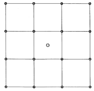
- Impurity or defect in a solid: An impurity or defect in a solid breaks the translational symmetry and, in principle, the methods we have discussed so far are not applicable. However, we can apply the above methods by choosing a large supercell and putting the impurity in the middle of the central cell as shown in Fig. 13.6. The figure shows a \(3\times3\) supercell in two dimensions. The unit cell of the periodic system is represented by a small square and the supercell consists of \(3\times3\) such unit cells. The impurity is placed in the central cell. The supercell is chosen large enough so that there is almost no interaction between two impurities in the neighboring supercells. This supercell becomes the unit cell for the calculation involving the impurity. Note that impurities can also be handled by using the Green’s function method as discussed in Chapter 8.
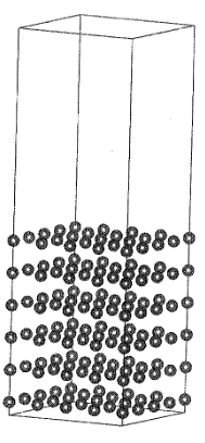
- Surface or interface: In this case, there is periodicity in the plane of the surface but there is no periodicity in the direction perpendicular to the surface. For the case when there is a vacuum on one side and solid on the other, a supercell is shown in Fig. 13.7. The supercell contains a crystal slab and vacuum region.
This is also called slab geometry. To represent the isolated surface accurately, one must ensure that
The width of the vacuum region must be wide enough so that the faces of the adjacent crystal slabs do not interact across the vacuum region.
The thickness of the crystal slab should be large enough so that the two surfaces of the crystal slab do not interact with each other. Similarly, an interface between the solids A and B can be handled. Now, instead of vacuum, one has a solid A or B.
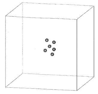
- Atomic cluster: An isolated cluster of atoms can also be handled by using a large supercell as shown in Fig. 13.8. The cluster is placed at the center of the supercell and the supercell is chosen to be large enough so that the two clusters in the neighboring supercells do not interact.
- Nanowire: A nanowire has length that is very large compared to its diameter, which is of the order of nanometers. This can be approximated by assuming that there is a periodicity along the length of the wire but no periodicity in the direction perpendicular to it. In Fig. 13.9, we show schematically the supercell geometry for the nanowire. The supercell is shown by solid lines. In directions perpendicular to the wire, there is vacuum. The width of this vacuum region should be large enough so that there is no interaction between the wires in the neighboring supercells.
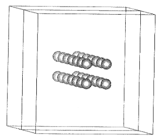
We see that the size of the supercell is much larger than the primitive cell of the solid. As a result, there is a high increase in the computing cost, which goes as \(\Omega_{cell}^3\), where \(\Omega_{cell}\) is the volume of the unit cell. For dealing with nonperiodic solids, one can develop specialized techniques that can handle nonperiodicity more efficiently (e.g., see Chapter 8). However, the pseudopotential technique is very efficient and at times it is more convenient to use the supercell technique rather than go for a specialized technique.
13.9 Exercises
Show that the phase-shift \(\delta_l(\varepsilon)\) can be written in terms of log derivatives \(\gamma_l\) as
\[ \delta_l(\varepsilon)=\cot^{-1}\left[\frac{k n_l'-\gamma_l n_l}{k j_l'-\gamma_l j_l}\right]_{r=r_m} \]
Show that the matrix element of the local part of the pseudopotential between plane waves \(\langle\vec k+\vec G|W^{loc}(\vec r)|\vec k+\vec G'\rangle\) is given by Eq. 13.44.
Show that the matrix element of the atomic nonlocal potential between plane waves \(\langle\vec k+\vec G|w^{nl}(\vec r,\vec r')|\vec k+\vec G'\rangle\) is given by Eq. 13.52.
Show that the local pseudopotential energy, \(E_{ps}^{loc}\), is given by Eq. 13.58.
Show that the nonlocal pseudopotential energy, \(E_{ps}^{nl}\), is given by Eq. 13.60.
Generate the atomic pseudopotential for copper in atomic configuration \(3d^{10}4s^1\) using one of the codes listed in Appendix A. Check the eigenvalues obtained by using the full potential and the pseudopotential. Compare (i) full potential and \(\ell=0\) and \(\ell=1\) components of the pseudopotential, and (ii) 4s wave function and \(\ell=0\) pseudowave function.
Generate the ultrasoft pseudopotential for copper using the codes listed in Appendix A and compare your results with the results obtained in Exercise 15.6.
Generate the atomic pseudopotential for silicon in its atomic ground state \(3s^23p^2\) using one of the codes listed in Appendix A. Check the eigenvalues obtained by using full potential and the pseudopotential. Compare (i) full potential and \(\ell=0\) and \(\ell=1\) components of the pseudopotential and (ii) 3s wave function and \(\ell=0\) pseudowave function.
Using the pseudopotential generated in Exercise 15.6 for Cu, calculate band structure, density of states, and charge density in (110) plane for Cu in fcc structure using one of the plane wave codes listed in Appendix A. Compare your results with the results shown in Chapter 4.
Using the pseudopotential generated in Exercise 15.8 for silicon, calculate band structure, density of states, and charge density in (110) plane for silicon in the diamond structure using one of the plane wave codes listed in Appendix A. Compare your results with the results shown in Chapter 4.
13.10 Further Reading
Ashcroft N. and Mermin N. 1976. Solid State Physics. New York: W. B. Saunders Company.
Harrison W. 1970. Solid State Theory. New York: McGraw-Hill Book Company.
Kaxiras E. 2003. Atomic and Electronic Structure of Solids. Cambridge: Cambridge University Press.
Kohanoff J. 2006. Electronic Structure Methods for Solids and Molecules. Cambridge: Cambridge University Press.
Martin R. M. 2004. Electronic Structure, Basic Theory and Practical Methods. Cambridge: Cambridge University Press.
Singh D. J. and Nordstrom L. 2006. Planewaves, Pseudopotentials, and the LAPW Method (Second Edition). New York: Springer.