7 Born-Oppenheimer Approximation
7.1 The many body problem
The time-independent Schrödinger equation for a system of electrons and nuclei:
\[ \hat{H}\Psi = E\Psi \tag{7.1}\]
The full many-body Hamiltonian (in atomic units \(\hbar = m_e = e = 1\)) is: \[ \begin{aligned} \hat{H} &= -\frac{1}{2}\sum_i \nabla_i^2 - \sum_{i,I} \frac{Z_I}{|\mathbf{r}_i - \mathbf{R}_I|} + \frac{1}{2}\sum_{i \neq j} \frac{1}{|\mathbf{r}_i - \mathbf{r}_j|} \\[6pt] &\quad - \sum_I \frac{\nabla_I^2}{2M_I} + \frac{1}{2}\sum_{I \neq J} \frac{Z_I Z_J}{|\mathbf{R}_I - \mathbf{R}_J|} \end{aligned} \tag{7.2}\]
where \(\mathbf{r}_i\) are electron coordinates, \(\mathbf{R}_I\) are nuclear coordinates, \(Z_I\) are atomic numbers, and \(M_I\) are nuclear masses.
7.2 The Born–Oppenheimer Approximation
Because nuclei are much heavier than electrons (\(M_I \gg m_e\)), they move much more slowly. We can therefore separate electronic and nuclear motion:
\[ \Psi(\mathbf{r}, \mathbf{R}) \approx \psi_e(\mathbf{r};\mathbf{R})\,\chi(\mathbf{R}) \tag{7.3}\]
The electronic Schrödinger equation at fixed nuclear positions \(\mathbf{R}\):
\[ \hat{H}_e\,\psi_e(\mathbf{r};\mathbf{R}) = E_e(\mathbf{R})\,\psi_e(\mathbf{r};\mathbf{R}) \tag{7.4}\]
The electronic energy \(E_e(\mathbf{R})\) as a function of nuclear positions defines the Born–Oppenheimer potential energy surface (BOPES), which plays the role of \(U(\mathbf{r})\) in Eq. 3.1.
The BOPES from Eq. 7.4 is what DFT (Chapter 5) computes, and what machine learning potentials (Chapter 7) learn to approximate. All forces in ab initio MD come from the gradient of this surface.
7.2.1 Physical Motivation
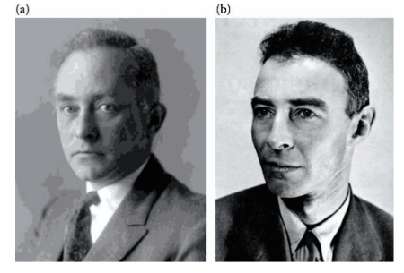
The Born–Oppenheimer approximation allows us to decouple the electronic and ionic motions. As a result, electrons and ions can be treated as nearly independent entities. Since the number of electrons and ions is very large \(\sim\!10^{24}\), an exact quantum mechanical solution of this problem is almost impossible. The Born–Oppenheimer approximation (Born and Oppenheimer 1927) (see Fig. 7.1) helps us in finding an approximate solution of this problem by separating electronic and ionic wave functions. The essential idea is that the ions, being \(10^3\)–\(10^5\) times heavier than the electrons, move much more slowly than the electrons. In other words, the timescale of electronic motion is much smaller than that of ionic motion. For example, the electronic velocities in a sodium metal are of the order of \(10^6\) m/s while the ions move with velocities of the order of \(10^2\) m/s. As a result, the electrons adjust very quickly to the motions of ions. Thus, when solving the electronic problem, we can assume that the ions are fixed at their instantaneous positions and the electrons follow the ionic motion adiabatically. We further assume that the electrons at any moment will be in their ground state for that particular instantaneous ionic configuration. In other words, the electrons are not allowed to make transitions from one state to another. Rather, they are assumed in their ground state and the ground state is deformed progressively by the ionic displacements.
7.2.2 The Full Many-Body Hamiltonian
Let \(\vec{r}_i\) denote the position of an electron, \(m_e\) the electronic mass, \(\vec{R}_\ell\) the ionic position, and \(M\) the ionic mass (Fig. 7.2). The Hamiltonian of the whole system of ions and electrons can be written as
\[ H = T_E + T_I + V_{II} + V_{EE} + V_{IE} \tag{7.5}\]
where \(T_E\) is the kinetic energy operator for electrons:
\[ T_E = -\sum_i \frac{\hbar^2}{2m_e} \frac{\partial^2}{\partial \vec{r}_i^{\,2}} \tag{7.6}\]
\(T_I\) is the kinetic energy operator for ions:
\[ T_I = -\sum_\ell \frac{\hbar^2}{2M} \frac{\partial^2}{\partial \vec{R}_\ell^{\,2}} \tag{7.7}\]
\(V_{II}\) is the ion–ion interaction:
\[ V_{II} = \frac{1}{2} \sum_{\substack{\ell,\ell' \\ \ell \neq \ell'}} \frac{e^2}{4\pi\varepsilon_0} \frac{Z_\ell Z_{\ell'}}{|\vec{R}_\ell - \vec{R}_{\ell'}|} \tag{7.8}\]
where \(Z_\ell e\) is the ionic charge at site \(\ell\). The factor of \(1/2\) avoids double counting. \(V_{EE}\) is the electron–electron interaction:
\[ V_{EE} = \frac{1}{2} \sum_{\substack{i,j \\ i \neq j}} \frac{1}{4\pi\varepsilon_0} \frac{e^2}{|\vec{r}_i - \vec{r}_j|} \tag{7.9}\]
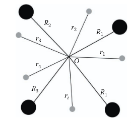
\(V_{IE}\) is the ion–electron interaction. We shall use \(r\) as the collective symbol for electronic coordinates, i.e. \(r \equiv (r_1, r_2, \ldots)\), and \(R\) as the collective symbol for ionic coordinates.
7.2.3 Wavefunction Decomposition
We are interested in finding the solution of the time-independent Schrödinger equation for the entire system of ions and electrons (Eq. 7.1). The Hamiltonian Eq. 7.5 contains all the interactions and would provide the theory of everything in materials science — provided we could solve it. To make progress, we try the following decomposition:
\[ \phi = \chi_I(\vec{R})\,\psi_E(r,\sigma,\vec{R}) \tag{7.10}\]
where \(\sigma\) is a composite symbol for the spins of the electrons. \(\psi_E\) represents the many-body electron wave function satisfying the Schrödinger equation with ions frozen at positions \(\vec{R}\):
\[ \bigl[T_E(r) + V_{EE}(r) + V_{IE}(r,\vec{R})\bigr]\,\psi_E(r,\vec{R}) = E_E(\vec{R})\,\psi_E(r,\vec{R}) \tag{7.11}\]
where \(E_E(\vec{R})\) is the energy of the electrons when the ions are frozen at position \(\vec{R}\), and \(\chi_I(\vec{R})\) is an ionic wave function yet to be determined.
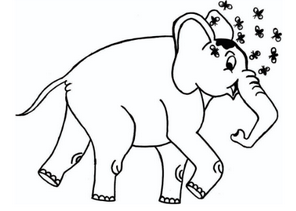
The physics behind this decomposition is that electrons, being light, move much faster than the ions and adjust their motion almost instantaneously. This is nicely illustrated in Fig. 7.3.
7.2.4 Derivation of the Ionic Equation
Substituting Eq. 7.10 into Eq. 7.1 and applying \(H\):
\[ \begin{aligned} H\phi &= \Bigl[ T_E(\vec{r}) + T_I(\vec{R}) + V_{II}(\vec{R}) + V_{EE}(\vec{r}) + V_{IE}(\vec{r},\vec{R}) \Bigr] \psi_E(\vec{r},\vec{R})\,\chi_I(\vec{R}) \\[6pt] &= \Bigl[ T_E(\vec{r}) + V_{EE}(\vec{r}) + V_{IE}(\vec{r},\vec{R}) \Bigr] \psi_E(\vec{r},\vec{R})\,\chi_I(\vec{R}) \\[4pt] &\quad + \left[ -\frac{\hbar^2}{2M} \sum_\ell \frac{\partial^2} {\partial \vec{R}_\ell^{\,2}} \right] \psi_E(\vec{r},\vec{R})\,\chi_I(\vec{R}) \\[4pt] &\quad + V_{II}(\vec{R})\, \psi_E(\vec{r},\vec{R})\,\chi_I(\vec{R}) \\[6pt] &= E\,\psi_E(\vec{r},\vec{R})\,\chi_I(\vec{R}) \end{aligned} \tag{7.12}\]
Expanding the second term:
\[ \begin{aligned} &-\frac{\hbar^2}{2M}\sum_\ell\left\{ \frac{\partial^2\psi_E}{\partial\vec{R}_\ell^{\,2}}\chi_I + 2\frac{\partial\psi_E}{\partial\vec{R}_\ell}\cdot\frac{\partial\chi_I}{\partial\vec{R}_\ell} + \psi_E\frac{\partial^2\chi_I}{\partial\vec{R}_\ell^{\,2}} \right\} + V_{II}\psi_E\chi_I \end{aligned} \tag{7.13}\]
Collecting terms, Eq. 7.12 becomes: \[ \begin{aligned} \Bigg[ -\frac{\hbar^2}{2M}\sum_\ell \frac{\partial^2}{\partial\vec{R}_\ell^{\,2}} + V_{II}(\vec{R}) + E_E(\vec{R}) \Bigg]\chi_I(\vec{R}) & \\ -\frac{\hbar^2}{2M}\sum_\ell \underbrace{ \left\{ \frac{\partial^2\psi_E}{\partial\vec{R}_\ell^{\,2}}\chi_I + 2\frac{\partial\psi_E}{\partial\vec{R}_\ell} \cdot \frac{\partial\chi_I}{\partial\vec{R}_\ell} \right\} }_{\text{neglected in BO approx.}} &= E\,\chi_I(\vec{R}) \end{aligned} \tag{7.14}\]
If the terms in the curly brackets can be neglected, \(\chi_I(\vec{R})\) satisfies:
\[ \boxed{ \left[-\frac{\hbar^2}{2M}\sum_\ell\frac{\partial^2}{\partial\vec{R}_\ell^{\,2}} + V_{II}(\vec{R}) + E_E(\vec{R})\right]\chi_I(\vec{R}) = E\,\chi_I(\vec{R}) } \tag{7.15}\]
This is the Schrödinger equation for the ions alone, with \(E_E(\vec{R})\) acting as an additional potential. It is clear from Eq. 7.15 that the binding of ions is provided by \(E_E(\vec{R})\), since \(V_{II}\) is purely repulsive. Thus, electrons form a glue that binds the ions.
7.2.5 Validity of the Neglected Terms
First term: The contribution involves \[ \begin{aligned} \int \psi_E^*\, \frac{\partial\chi_I}{\partial\vec{R}} \cdot \frac{\partial\psi_E}{\partial\vec{R}} \, d^3r &\approx \frac{\partial\chi_I}{\partial\vec{R}} \cdot \frac{1}{2} \frac{\partial}{\partial\vec{R}} \int \psi_E^*\psi_E\, d^3r \\[6pt] &= \frac{\partial\chi_I}{\partial\vec{R}} \cdot \frac{1}{2} \frac{\partial N_E}{\partial\vec{R}} = 0 \end{aligned} \tag{7.16}\]
since \(N_E = \int\psi_E^*\psi_E\,d^3r\) is the total number of electrons, which is constant — it does not change as a result of ionic motion.
Second term: In the extreme case of electrons tightly bound to their ions, \(\psi(\{r_i,\vec{R}\}) = \psi(\{r_i - \vec{R}\})\), which gives
\[ \frac{\partial^2\psi(\{r_i - \vec{R}\})}{\partial\vec{R}^2} = \frac{\partial^2\psi(\{r_i - \vec{R}\})}{\partial r_i^2} \tag{7.17}\]
The contribution to the expectation value of the energy then becomes
\[ -\int\psi_E^*\,\frac{\hbar^2}{2M}\frac{\partial^2\psi_E}{\partial\vec{R}^2}\,d^3r = \frac{m_e}{M}\left(-\int\psi_E^*\,\frac{\hbar^2}{2m_e}\frac{\partial^2\psi_E}{\partial r_i^2}\,d^3r\right) \tag{7.18}\]
This is \(m_e/M \sim 10^{-4}\)–\(10^{-5}\) times the kinetic energy of the electrons — entirely negligible.
Thus the decomposition Eq. 7.10 is indeed a good approximation. The first factor \(\chi_I(\vec{R})\) describes the ionic motion; the second factor \(\psi_E\) shows that electrons move as if the ions were fixed at their instantaneous positions. The electron follows the ionic motion adiabatically.
7.2.6 Born–Oppenheimer Potential Energy Surface
The decomposition Eq. 7.10 can be generalized to include a complete set of electronic wave functions:
\[ \phi = \sum_n \chi_I^n(\vec{R})\,\psi_{nE}(r,\vec{R}) \tag{7.19}\]
where \(n = 0\) is the electronic ground state. In the Born–Oppenheimer approximation we neglect the off-diagonal transitions between states — we assume that nuclear motion cannot cause electronic transitions and the electrons always remain in their ground state.
The quantity \(E_E^n(\vec{R}) + V_{II}(\vec{R})\) in Eq. 7.15 defines a surface in the space spanned by nuclear coordinates: the Born–Oppenheimer Potential Energy Surface (BOPES). For each electronic state \(n\) there is a separate BOPES. Normally we take \(n = 0\) (ground state), so the ions move on \(E_E^0(\vec{R}) + V_{II}(\vec{R})\) without making transitions to surfaces with \(n \neq 0\).
The BOPES from Eq. 7.4 is what DFT (Chapter 5) computes, and what machine learning potentials (Chapter 7) learn to approximate. All forces in ab initio MD come from the gradient of this surface.