12 Methods of Electronic Structure Calculations I
12.1 Introduction
In this chapter, we shall solve the KS equation for some simple models and try to understand the origin of the band gap. We shall then discuss the basic ideas of some well-known methods of band structure calculations such as the plane wave expansion method, the tight-binding model, the orthogonalized plane wave (OPW) method, and the pseudopotential method. We shall start with the empty lattice approximation in Section 12.2, which is the limiting case of effective potential approaching zero value. In Section 12.3, we shall then solve the KS equation for a weak effective potential, which is called the nearly free electron (NFE) model. In Section 12.4 and Section 12.5, we shall discuss the plane wave expansion and the tight-binding methods. The tight-binding method provides another way to look at how the bands are formed when atoms are brought from infinite distance to form a solid. In Section 12.6, we shall briefly discuss the Hubbard model, which is an attempt to incorporate electron correlations in solids. In Section 12.7, we shall briefly discuss Wannier functions, which are orthogonal localized functions centered on atomic sites. In Section 12.8, we shall discuss the OPW method, which led to the idea of pseudopotential. In Section 12.9, we shall discuss the pseudopotential method, which has emerged as a very powerful tool for calculating band structure, total energy, and structural and other properties of solids. In this chapter, we shall only discuss the basic idea of pseudopotential and the method will be discussed in more detail in the next chapter.
12.2 Empty Lattice Approximation
If the effective potential in the KS equation is reduced to zero, eigenvalues \(\varepsilon_{\vec{k}}\) of a solid approach the free electron values
\[ \varepsilon_{\vec{k}} = \frac{\hbar^2 k^2}{2m_e} \tag{12.1}\]
The wave vector \(\vec{k}\) in Eq. 12.1 is unrestricted and can vary from \(-\infty\) to \(+\infty\). However, we know that if we have a periodic lattice, all values of \(\vec{k}\) lie within the first BZ. Thus, if a wave vector \(\vec{k}'\) lies outside the BZ boundary, it has to be folded back within the first BZ by adding (or subtracting) a suitable reciprocal vector such that
\[ \vec{k}' = \vec{k} + \vec{G} \]
and
\[ \varepsilon_{\vec{k}'} = \varepsilon_{\vec{k}+\vec{G}} = \frac{\hbar^2}{2m_e}(\vec{k} + \vec{G})^2 \tag{12.2}\]
Thus, \(\varepsilon_{\vec{k}+\vec{G}}\) appears as a higher band at the wave vector \(\vec{k}\) than \(\varepsilon_{\vec{k}}\) in the first BZ. These bands are known as empty lattice bands. Here, “empty lattice” means that the effective potential is zero and in that sense the lattice is empty, that is, no atoms at the lattice points. The empty lattice approximation provides a good test for any method of calculating band structure; therefore, it is also known as the empty lattice test. The empty lattice bands provide a feel for the band structure, although the actual band structure will be quite different from it. Thus, by comparing it with the actual band structure of a solid, one can get some idea of the free electron nature of the bands.
To give an example, we first consider a one-dimensional lattice of lattice constant \(a\). The reciprocal lattice vectors are \(\pm(2\pi/a)n\). Therefore, the empty lattice bands are given by
\[ \varepsilon_{n\vec{k}} = \frac{\hbar^2}{2m_e}\left(k \pm \frac{2\pi}{a}\,n\right)^2 \tag{12.3}\]
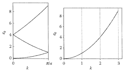
These bands are plotted in Fig. 12.1 and compared with the free electron bands. The way in which the “empty lattice” bands are plotted on left in Fig. 12.1 is known as the “reduced zone” scheme, in which the wave vector \(\vec{k}\) is restricted up to the first BZ boundary. Sometimes, it may be more useful to unfold the bands and plot them like free electron bands (right side) such that \(\vec{k}\) is unrestricted. This scheme is known as the “extended zone” scheme.
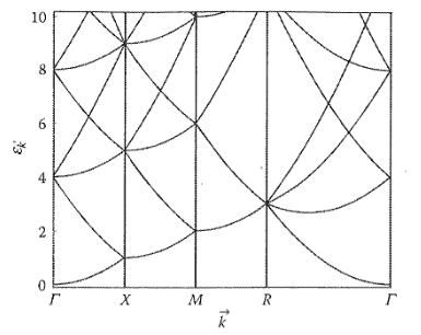
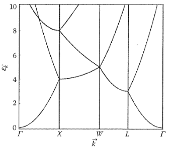
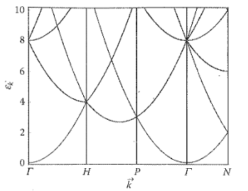
For simple cubic, fcc, and bcc solids, the calculation of empty lattice bands is left as an exercise but the results are shown in Fig. 12.2 through Fig. 12.4. The energy is given in units of \((\hbar\pi)^2/(2m_e a^2)\), where \(a\) is the cube edge.
12.3 Nearly Free Electron (NFE) Model
We saw that for \(v_{\text{eff}}(\vec{r}) = 0\), the solutions are plane waves. So, if the potential \(v_{\text{eff}}(\vec{r})\) is very weak, we can use perturbation theory to find the solution of the KS equation.
The Hamiltonian \(H\) can be written as
\[ H = -\frac{\hbar^2}{2m_e}\nabla^2 + v_{\text{eff}}(\vec{r}) = H_0 + v_{\text{eff}}(\vec{r}) \tag{12.4}\]
where \(H_0\) is the free electron Hamiltonian. The unperturbed eigenvectors and energy eigenvalues are
\[ \left|\vec{k}\right\rangle = \frac{1}{\sqrt{\Omega}}\,e^{i\vec{k}\cdot\vec{r}} \tag{12.5}\]
and
\[ \varepsilon_{\vec{k}}^0 = \frac{\hbar^2 k^2}{2m_e} \tag{12.6}\]
where \(\Omega\) is the volume of the solid. As \(v_{\text{eff}}(\vec{r})\) is weak, we treat it as a perturbation over \(H_0\). Using the second-order perturbation theory, the energy and the wave function of the perturbed electron are given by
\[ \varepsilon_{\vec{k}} = \varepsilon_{\vec{k}}^0 + \left\langle\vec{k}\left|v_{\text{eff}}\right|\vec{k}\right\rangle + \sum_{\vec{k}'\neq\vec{k}}\frac{\left|\left\langle\vec{k}\left|v_{\text{eff}}\right|\vec{k}'\right\rangle\right|^2}{\varepsilon_{\vec{k}}^0 - \varepsilon_{\vec{k}'}^0} \tag{12.7}\]
and
\[ \psi_{\vec{k}}(\vec{r}) = \left|\vec{k}\right\rangle + \sum_{\vec{k}'\neq\vec{k}}\frac{\left\langle\vec{k}'\left|v_{\text{eff}}\right|\vec{k}\right\rangle}{\varepsilon_{\vec{k}}^0 - \varepsilon_{\vec{k}'}^0}\left|\vec{k}'\right\rangle \tag{12.8}\]
where
\[ \left\langle\vec{k}\left|v_{\text{eff}}\right|\vec{k}'\right\rangle = \frac{1}{\Omega}\int v_{\text{eff}}(\vec{r})\,e^{-i(\vec{k}-\vec{k}')\cdot\vec{r}}\,d^3r \tag{12.9}\]
Since \(v_{\text{eff}}(\vec{r})\) is periodic in \(\vec{r}\), it can be expanded as
\[ v_{\text{eff}}(\vec{r}) = \sum_{\vec{G}}v(\vec{G})\exp(i\vec{G}\cdot\vec{r}) \tag{12.10}\]
where \(\vec{G}\) is a reciprocal lattice vector and the sum is over all the reciprocal lattice vectors. Since \(v_{\text{eff}}(\vec{r})\) is real
\[ v^*(\vec{G}) = v(-\vec{G}) \tag{12.11}\]
Substituting Eq. 12.10 in Eq. 12.9, we get
\[ \left\langle\vec{k}\left|v_{\text{eff}}\right|\vec{k}'\right\rangle = \frac{1}{\Omega}\sum_{\vec{G}}v(\vec{G})\int e^{-i(\vec{k}-\vec{k}'-\vec{G})\cdot\vec{r}}\,d^3r \tag{12.12}\]
Using the identity
\[ \int e^{i\vec{k}\cdot\vec{r}}\,d^3r = \Omega\,\delta_{\vec{k},0} \tag{12.13}\]
we get
\[ \left\langle\vec{k}\left|v_{\text{eff}}\right|\vec{k}'\right\rangle = \begin{cases} v(\vec{G}) & \text{if } \vec{k} - \vec{k}' = \vec{G} = \text{a reciprocal lattice vector} \\ 0 & \text{otherwise} \end{cases} \tag{12.14}\]
Using Eq. 12.7, Eq. 12.11, and Eq. 12.14, we get
\[ \varepsilon_{\vec{k}} = \varepsilon_{\vec{k}}^0 + v(0) + \sum_{\vec{G}\neq 0}\frac{\left|v(\vec{G})\right|^2}{\varepsilon_{\vec{k}}^0 - \varepsilon_{\vec{k}-\vec{G}}^0} \tag{12.15}\]
and
\[ \psi_{\vec{k}}(\vec{r}) = \left|\vec{k}\right\rangle + \sum_{\vec{G}\neq 0}\frac{v(-\vec{G})}{\varepsilon_{\vec{k}}^0 - \varepsilon_{\vec{k}-\vec{G}}^0}\left|\,(\vec{k}-\vec{G})\right\rangle \tag{12.16}\]
Eq. 12.15 and Eq. 12.16 will give meaningful results only if the expansion in the reciprocal space converges rapidly. This implies that the coefficients \(v(\vec{G})\) should fall off very rapidly as \(\vec{G}\) increases. Also, there should be no degeneracy between the unperturbed states, that is, \(\varepsilon_{\vec{k}}^0 \neq \varepsilon_{\vec{k}-\vec{G}}^0\). Thus, our perturbation expansion will break down if
\[ \left|\vec{k}\right| = \left|\vec{k} - \vec{G}\right| \tag{12.17}\]
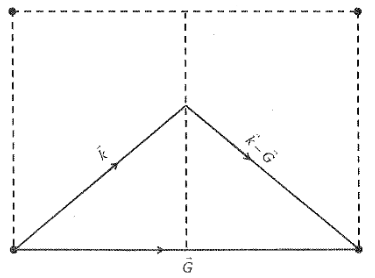
This condition can be shown geometrically as in Fig. 12.5. The figure shows that condition (Eq. 12.17) will hold if \(\vec{k}\) lies on the perpendicular bisector plane of \(\vec{G}\). But these bisector planes define the boundaries of the BZ. Thus, our perturbation expansion will break down near the zone boundary. We note that Eq. 12.17 is the Laue condition of x-ray diffraction (see, e.g., Ashcroft and Mermin 1976). The Laue condition is a consequence of wave propagation in crystals. So, what we have obtained is essentially a consequence of the wave nature of electrons.
So, what is happening near the zone boundary is a strong interference of incoming wave \(|\vec{k}\rangle\) and diffracted wave \(|\vec{k} - \vec{G}\rangle\). In Eq. 12.16, it is implicitly assumed that the coefficient of \(|\vec{k} - \vec{G}\rangle\) is much smaller than the coefficient of \(|\vec{k}\rangle\). But near the zone boundary, this assumption breaks down; therefore, we must treat all the coefficients on an equal footing, implying that \(\psi_{\vec{k}}(\vec{r})\) should be expanded as
\[ \psi_{\vec{k}}(\vec{r}) = \sum_{\vec{G}}C_{\vec{k}-\vec{G}}\left|\vec{k}-\vec{G}\right\rangle \tag{12.18}\]
\[ = \frac{1}{\Omega^{1/2}}\sum_{\vec{G}}C_{\vec{k}-\vec{G}}\,e^{i(\vec{k}-\vec{G})\cdot\vec{r}} \tag{12.19}\]
This is because the periodic potential \(v_{\text{eff}}(\vec{r})\) can mix only those plane waves with \(\vec{k}\) vectors differing by a reciprocal vector \(\vec{G}\) (see Eq. 12.14). For the sake of illustration, let us retain only two terms in the expansion (Eq. 12.18), that is
\[ \psi_{\vec{k}}(\vec{r}) = C_{\vec{k}}\left|\vec{k}\right\rangle + C_{\vec{k}-\vec{G}}\left|\vec{k}-\vec{G}\right\rangle \tag{12.20}\]
Let us substitute it in the KS equation
\[ \left[\frac{-\hbar^2}{2m_e}\nabla^2 + v_{\text{eff}}(\vec{r})\right]\psi_{\vec{k}}(\vec{r}) = \varepsilon_{\vec{k}}\psi_{\vec{k}}(\vec{r}) \tag{12.21}\]
We get
\[ \begin{aligned} C_{\vec{k}}\,\varepsilon_{\vec{k}}^0\left|\vec{k}\right\rangle + C_{\vec{k}-\vec{G}}\,\varepsilon_{\vec{k}-\vec{G}}^0\left|\vec{k}-\vec{G}\right\rangle &+ C_{\vec{k}}\,v_{\text{eff}}(\vec{r})\left|\vec{k}\right\rangle + C_{\vec{k}-\vec{G}}\,v_{\text{eff}}(\vec{r})\left|\vec{k}-\vec{G}\right\rangle \\ &= \varepsilon_{\vec{k}}\!\left(C_{\vec{k}}\left|\vec{k}\right\rangle + C_{\vec{k}-\vec{G}}\left|\vec{k}-\vec{G}\right\rangle\right) \end{aligned} \tag{12.22}\]
By multiplying Eq. 12.22 by \(\langle\vec{k}'|\) from the left, we get
\[ \begin{aligned} C_{\vec{k}}\,\varepsilon_{\vec{k}}^0\,\delta_{\vec{k}',\vec{k}} + C_{\vec{k}-\vec{G}}\,\varepsilon_{\vec{k}-\vec{G}}^0\,\delta_{\vec{k}',\vec{k}-\vec{G}} &+ C_{\vec{k}}\,v(\vec{k}'-\vec{k}) + C_{\vec{k}-\vec{G}}\,v(\vec{k}'-\vec{k}+\vec{G}) \\ &= \varepsilon_{\vec{k}}\,C_{\vec{k}}\,\delta_{\vec{k}',\vec{k}} + \varepsilon_{\vec{k}}\,C_{\vec{k}-\vec{G}}\,\delta_{\vec{k}',\vec{k}-\vec{G}} \end{aligned} \tag{12.23}\]
Eq. 12.23 gives two equations, one for \(\vec{k}' = \vec{k}\) and the other for \(\vec{k}' = \vec{k} - \vec{G}\). Using Eq. 12.14 and setting \(v(0) = 0\), we get
\[ \begin{aligned} \left(\varepsilon_{\vec{k}}^0 - \varepsilon_{\vec{k}}\right)C_{\vec{k}} + C_{\vec{k}-\vec{G}}\,v(\vec{G}) &= 0 \\ v(-\vec{G})\,C_{\vec{k}} + \left(\varepsilon_{\vec{k}-\vec{G}}^0 - \varepsilon_{\vec{k}}\right)C_{\vec{k}-\vec{G}} &= 0 \end{aligned} \tag{12.24}\]
Eq. 12.24 will have a nontrivial solution only if
\[ \begin{vmatrix} \varepsilon_{\vec{k}}^0 - \varepsilon_{\vec{k}} & v(\vec{G}) \\ v^*(\vec{G}) & \varepsilon_{\vec{k}-\vec{G}}^0 - \varepsilon_{\vec{k}} \end{vmatrix} = 0 \tag{12.25}\]
This gives a quadratic equation in \(\varepsilon_{\vec{k}}\), which has two roots given by
\[ \varepsilon_{\vec{k}}^{\pm} = \frac{1}{2}\left[\left(\varepsilon_{\vec{k}}^0 + \varepsilon_{\vec{k}-\vec{G}}^0\right) \pm \left\{\left(\varepsilon_{\vec{k}}^0 - \varepsilon_{\vec{k}-\vec{G}}^0\right)^2 + 4\left|v(\vec{G})\right|^2\right\}^{1/2}\right] \tag{12.26}\]
At the zone boundary, \(|\vec{k}| = |\vec{k} - \vec{G}|\), and \(\varepsilon_{\vec{k}}^0 = \varepsilon_{\vec{k}-\vec{G}}^0\), so that from Eq. 12.26, we get
\[ \varepsilon_{\vec{k}}^{\pm} = \varepsilon_{\vec{k}}^0 \pm \left|v(\vec{G})\right| \tag{12.27}\]
So, at the zone boundary, we get a gap of \(2|v(\vec{G})|\) between the energies of the states \(\psi_{\vec{k}}^+(\vec{r})\) and \(\psi_{\vec{k}}^-(\vec{r})\). At the zone center, that is, \(\vec{k} = 0\), \(\varepsilon_{\vec{k}}^0 - \varepsilon_{\vec{k}-\vec{G}}^0\) is very large compared to \(|v(\vec{G})|\), so that
\[ \begin{aligned} \varepsilon_{\vec{k}}^+ &= \varepsilon_{\vec{k}-\vec{G}}^0 \\ \varepsilon_{\vec{k}}^- &= \varepsilon_{\vec{k}}^0 \end{aligned} \tag{12.28}\]
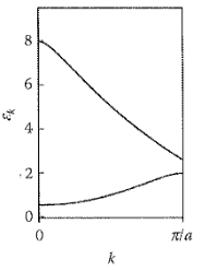
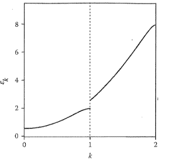
Thus, the effect of perturbation is quite small at \(\vec{k}\) points far away from the zone boundary; therefore, \(\varepsilon_{\vec{k}}\) will remain close to a parabolic shape. For the one-dimensional case, \(\varepsilon_{\vec{k}}\) is schematically shown in Fig. 12.6. The same result is shown in the extended zone scheme in Fig. 12.7, which shows more clearly how \(\varepsilon_{\vec{k}}\) are obtained by perturbing the free electron energies \(\varepsilon_{\vec{k}}^0\). From these figures, it is clear that there are some values of energy for which there are no allowed electron states and the one-electron energy spectrum has gaps. This is essentially the consequence of the wave nature of electrons, which gives rise to Bragg diffraction at the zone boundaries. We shall further discuss this from a different point of view when discussing the tight-binding method.
It turns out that the energy bands of several alkali metals such as Mg, Zn, Al, and so on resemble the NFE bands. This raises two very important questions. First, how can we view the electrons, which interact via Coulomb potential, as noninteracting particles? Second, how can we assume that the electron–ion interaction is weak? Landau answered the first question using the Fermi liquid theory (Landau 1957, 1959). The theory explains why some properties of the interacting electron gas resemble that of weakly interacting quasi-particles. We saw that the density functional theory also reduced the many-body problem by mapping it onto a system of noninteracting electrons. The second question is answered using the pseudopotential theory as we shall see later in this chapter.
12.4 Plane Wave Expansion Method
In the above treatment, we had included only two plane waves in the expansion of \(\psi_{\vec{k}}(\vec{r})\) in Eq. 12.20. We can generalize the above treatment to the case where many plane waves are included in the expansion, that is
\[ \psi_{\vec{k}}(\vec{r}) = \sum_{\vec{G}}C_{\vec{k}-\vec{G}}\left|\vec{k}-\vec{G}\right\rangle \tag{12.29}\]
Substituting this in Eq. 12.21, we will get a set of equations, similar to Eq. 12.24, that is
\[ \left(\varepsilon_{\vec{k}-\vec{G}}^0 - \varepsilon_{\vec{k}}\right)C_{\vec{k}-\vec{G}} + \sum_{\vec{G}'}v(\vec{G}'-\vec{G})\,C_{\vec{k}-\vec{G}'} = 0 \tag{12.30}\]
These equations will have nontrivial solutions only if
\[ \det\!\left|\left(\varepsilon_{\vec{k}-\vec{G}}^0 - \varepsilon_{\vec{k}}\right)\delta_{\vec{G},\vec{G}'} + v(\vec{G}'-\vec{G})\right| = 0 \tag{12.31}\]
We can obtain the band structure, that is, \(\varepsilon_{\vec{k}}\) versus \(\vec{k}\) by solving this equation. The expansion (Eq. 12.29) is called the plane wave expansion and the method the plane wave expansion method. In principle, Eq. 12.31 is exact but then one should take infinite number of plane waves in the expansion (Eq. 12.29). Thus, the suitability of the method for practical calculations depends on the size of the determinant in Eq. 12.31, which in turn depends on how quickly \(v(\vec{G})\) falls as \(\vec{G}\) increases. If we look at Figure 4.1, we note that \(v_{\text{eff}}(\vec{r})\) has sharp variations near the ions, that is, when \(\vec{r}\) is small. This would imply that its Fourier components will be large for large \(\vec{G}\) and would not fall quickly as \(\vec{G}\) increases, in general. Thus, the method is not suitable for practical calculation if one uses the actual potential, but if one uses the pseudopotential instead, this method is very efficient and useful, as we shall see later.
It should be noted that \(\psi_{\vec{k}}(\vec{r})\) given by Eq. 12.29 satisfies Bloch’s theorem. This can be viewed as an alternate proof of Bloch’s theorem.
12.5 Tight-Binding Method
We just saw how energy bands are formed when the electrons move in a weak periodic potential. Now, we shall look into this problem from a different point of view. We shall try to understand how energy bands are formed when atoms are brought closer, to form a crystal.
Let us suppose that we are given a large number of sodium atoms and we wish to form a solid using these atoms. We first arrange these atoms on a bcc lattice with a large lattice spacing (say 1 mm) and then slowly squeeze this system of atoms, retaining the lattice structure. When the atoms are far apart, all the electrons are localized at their respective atoms and there is a negligible overlap between the wave functions of two electrons on the neighboring sites. As we decrease the lattice spacing, the overlap between the wave functions of the outermost electrons on the neighboring atoms begins to increase. This overlap will be considerable when the lattice spacing is reduced to small values, say about the lattice constant of sodium. Now, an outermost 3s electron is no longer localized on a particular atom, but has a good probability of jumping on to other atoms. Therefore, a single atomic orbital \(\phi_a(\vec{r})\) cannot represent this electron; rather, we should form a linear combination of atomic orbitals centered on different sites for its correct description, that is
\[ \psi_{\vec{k}}(\vec{r}) = \sum_\ell C_{\vec{k}\ell}\,\phi_a(\vec{r} - \vec{R}_\ell) \tag{12.32}\]
For simplicity, we assume \(\phi_a(\vec{r})\) to be a nondegenerate state such as s-state. Generalization to include more states will be done later.
Because \(\psi_{\vec{k}}(\vec{r})\) in Eq. 12.32 represents a wave function of an electron in a solid, it must satisfy Bloch’s theorem, that is
\[ \psi_{\vec{k}}(\vec{r} + \vec{R}) = e^{i\vec{k}\cdot\vec{R}}\,\psi_{\vec{k}}(\vec{r}) \tag{12.33}\]
This is satisfied only if \(C_{\vec{k}\ell} = e^{i\vec{k}\cdot\vec{R}_\ell}\), so that
\[ \psi_{\vec{k}}(\vec{r}) = \sum_\ell e^{i\vec{k}\cdot\vec{R}_\ell}\,\phi_a(\vec{r} - \vec{R}_\ell) \tag{12.34}\]
As a first approximation, the energy \(\varepsilon_{\vec{k}}\) of the state \(\psi_{\vec{k}}(\vec{r})\) is given by the expectation value of Hamiltonian \(H\), that is
\[ \varepsilon_{\vec{k}} = \frac{\displaystyle\int\psi_{\vec{k}}^*(\vec{r})\left[-\frac{\hbar^2}{2m_e}\nabla^2 + v(\vec{r})\right]\psi_{\vec{k}}(\vec{r})\,d^3r}{\displaystyle\int\psi_{\vec{k}}^*(\vec{r})\psi_{\vec{k}}(\vec{r})\,d^3r} \tag{12.35}\]
Using Eq. 12.34, the denominator in Eq. 12.35 can be written as
\[ \begin{aligned} \int\psi_{\vec{k}}^*(\vec{r})\psi_{\vec{k}}(\vec{r})\,d^3r &= \sum_{\ell\ell'}e^{i\vec{k}\cdot(\vec{R}_\ell - \vec{R}_{\ell'})}\int\phi_a^*(\vec{r}-\vec{R}_{\ell'})\,\phi_a(\vec{r}-\vec{R}_\ell)\,d^3r \\ &= \sum_\ell\int\left|\phi_a(\vec{r}-\vec{R}_\ell)\right|^2 d^3r + \sum_{\substack{\ell\,\ell' \\ \ell'\neq\ell}}e^{i\vec{k}\cdot(\vec{R}_\ell - \vec{R}_{\ell'})} \\ &\quad\times\int\phi_a^*(\vec{r}-\vec{R}_{\ell'})\,\phi_a(\vec{r}-\vec{R}_\ell)\,d^3r \end{aligned} \tag{12.36}\]
Since \(\phi_a(\vec{r})\) are atomic orbitals, the overlap between the atomic orbitals centered on different sites will be small as compared to \(|\phi_a(\vec{r})|^2\); therefore, we neglect the second term in Eq. 12.36. Also
\[ \int\left|\phi_a(\vec{r}-\vec{R}_\ell)\right|^2 d^3r = \int|\phi_a(\vec{r})|^2\,d^3r = 1 \tag{12.37}\]
Thus, from Eq. 12.36, we get
\[ \int\psi_{\vec{k}}^*(\vec{r})\psi_{\vec{k}}(\vec{r})\,d^3r = \sum_\ell 1 = N \]
where \(N\) is the total number of atoms in the solid. Eq. 12.35 can now be written as
\[ \varepsilon_{\vec{k}} = \frac{1}{N}\sum_{\ell\ell'}e^{i\vec{k}\cdot(\vec{R}_\ell - \vec{R}_{\ell'})}\int\phi_a^*(\vec{r}-\vec{R}_{\ell'})\left[-\frac{\hbar^2}{2m_e}\nabla^2 + v(\vec{r})\right]\phi_a(\vec{r}-\vec{R}_\ell)\,d^3r \]
Let us write \(\vec{R}_\ell - \vec{R}_{\ell'} = \vec{R}_j\) or \(\vec{R}_{\ell'} = \vec{R}_\ell - \vec{R}_j\). Thus
\[ \varepsilon_{\vec{k}} = \frac{1}{N}\sum_j e^{i\vec{k}\cdot\vec{R}_j}\sum_\ell\int\phi_a^*(\vec{r}-\vec{R}_\ell+\vec{R}_j)\left[-\frac{\hbar^2}{2m_e}\nabla^2 + v(\vec{r})\right]\phi_a(\vec{r}-\vec{R}_\ell)\,d^3r \tag{12.38}\]
Because Hamiltonian \(H\) is translationally invariant, the integral in Eq. 12.38 will depend only on the relative distance between the two sites on which the orbitals are centered. Thus, for a fixed \(j\), the integral in Eq. 12.38 is the same for each \(\ell\). Therefore, the summation over \(\ell\) in Eq. 12.38 simply gives a multiplicative factor \(N\). Thus, Eq. 12.38 can be written as
\[ \varepsilon_{\vec{k}} = \sum_j e^{i\vec{k}\cdot\vec{R}_j}\,\varepsilon_j \tag{12.39}\]
where
\[ \varepsilon_j = \int\phi_a^*(\vec{r}+\vec{R}_j)\left[-\frac{\hbar^2}{2m_e}\nabla^2 + v(\vec{r})\right]\phi_a(\vec{r})\,d^3r \tag{12.40}\]
Eq. 12.39 proves a very general point regarding the energy bands. It shows that the energy bands are periodic in reciprocal space, that is
\[ \varepsilon_{\vec{k}+\vec{G}} = \varepsilon_{\vec{k}} \tag{12.41}\]
where \(\vec{G}\) is a reciprocal lattice vector. This means the band structure is repeated as you go from one cell of the reciprocal space to another. Sometimes, it may be useful to plot the band structure in this way, which is known as the “repeated zone scheme.”
Let \(H_a\) be the Hamiltonian for an isolated single atom with atomic potential \(v_a(\vec{r})\), that is
\[ H_a = -\frac{\hbar^2}{2m_e}\nabla^2 + v_a(\vec{r}) \tag{12.42}\]
and \(\phi_a(\vec{r})\) be the solution of the equation
\[ H_a\,\phi_a(\vec{r}) = \varepsilon_a\,\phi_a(\vec{r}) \tag{12.43}\]
where \(\varepsilon_a\) is the atomic energy level. Now, let us evaluate the integral in Eq. 12.40 in terms of \(\varepsilon_a\). Thus
\[ \begin{aligned} \left[-\frac{\hbar^2}{2m_e}\nabla^2 + v(\vec{r})\right]\phi_a(\vec{r}) &= \left[-\frac{\hbar^2}{2m_e}\nabla^2 + v_a(\vec{r})\right]\phi_a(\vec{r}) + \left[v(\vec{r}) - v_a(\vec{r})\right]\phi_a(\vec{r}) \\ &= \varepsilon_a\,\phi_a(\vec{r}) + \left[v(\vec{r}) - v_a(\vec{r})\right]\phi_a(\vec{r}) \end{aligned} \tag{12.44}\]
Substituting Eq. 12.44 into Eq. 12.39, we get
\[ \begin{aligned} \varepsilon_{\vec{k}} &= \sum_j e^{i\vec{k}\cdot\vec{R}_j}\int\phi_a^*(\vec{r}+\vec{R}_j)\left[\varepsilon_a\,\phi_a(\vec{r}) + \left\{v(\vec{r}) - v_a(\vec{r})\right\}\phi_a(\vec{r})\right]d^3r \\ &= \varepsilon_0 + \sum_{j\neq 0}e^{i\vec{k}\cdot\vec{R}_j}\,\gamma_j \end{aligned} \tag{12.45}\]
where
\[ \varepsilon_0 = \varepsilon_a + \int\phi_a^*(\vec{r})\left[v(\vec{r}) - v_a(\vec{r})\right]\phi_a(\vec{r})\,d^3r \tag{12.46}\]
and
\[ \gamma_j = \int\phi_a^*(\vec{r}+\vec{R}_j)\left[v(\vec{r}) - v_a(\vec{r})\right]\phi_a(\vec{r})\,d^3r \tag{12.47}\]
Here, \(\gamma_j\) is called overlap integral or hopping integral. For an s-state, \(\phi_a(\vec{r})\) depends only on the magnitude of \(\vec{r}\) and thus, \(\gamma_j = \gamma_{-j}\). Also, for simplicity, let us neglect all the overlap integrals except the nearest-neighbor integrals. Thus, Eq. 12.45 can be written as
\[ \varepsilon_{\vec{k}} = \varepsilon_0 + \sum_{\substack{j\neq 0 \\ nn}}\gamma_j\,e^{i\vec{k}\cdot\vec{R}_j} \tag{12.48}\]
where \(nn\) indicates that the sum is only over the nearest neighbors.
Let us evaluate Eq. 12.48 for a simple cubic lattice. We have six nearest neighbors at \((\pm a,0,0)\), \((0,\pm a,0)\), and \((0,0,\pm a)\) positions, where \(a\) is the lattice constant. Thus, \(\varepsilon_{\vec{k}}\) for a simple cubic lattice are given by
\[ \begin{aligned} \varepsilon_{\vec{k}} &= \varepsilon_0 + \gamma\left[e^{ik_x a} + e^{-ik_x a} + e^{ik_y a} + e^{-ik_y a} + e^{ik_z a} + e^{-ik_z a}\right] \\ &= \varepsilon_0 + 2\gamma\left(\cos k_x a + \cos k_y a + \cos k_z a\right) \end{aligned} \tag{12.49}\]
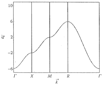
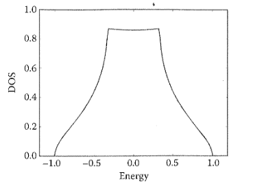
\(\varepsilon_{\vec{k}}\) versus \(\vec{k}\) curve for a simple cubic lattice for \(\vec{k}\) along various symmetry directions in the BZ is shown in Fig. 12.8. We see that the band is flatter near the zone boundary and near the zone center as was the case with the NFE model. The bandwidth in this case is \(12\gamma\). In general, if there are \(z\) nearest neighbors, the bandwidth in tight-binding approximation is \(2z\gamma\). If \(\gamma\) is large, we have a broadband, and if \(\gamma\) is small, we get a narrow band. Since \(\gamma\) increases by decreasing lattice spacing \(a\), the band will get broader as we decrease \(a\). The density of states (DOS) for a cubic single-band tight-binding model is shown in Fig. 12.9. One can clearly see the van Hove singularities in the DOS around energies \(\varepsilon = -1\), \(-0.4\), \(0.4\), and \(1.0\).
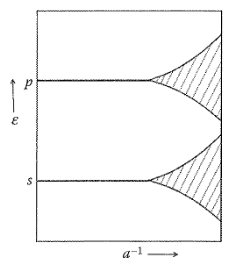
Based on the above discussion, we can now answer the question with which we started, that is, how energy bands are formed when the atoms are brought together to form a solid. When the atoms are far apart, the electrons are localized at the atoms with energies \(\varepsilon_1\), \(\varepsilon_2\), and so on. When the atoms are brought closer, the atomic wave functions centered on different sites begin to overlap and the atomic levels \(\varepsilon_1\), \(\varepsilon_2\), and so on begin to broaden to form energy bands as shown in Fig. 12.10. The bands are, therefore, sometimes labeled as \(s\)-band, \(d\)-band, and so on to identify the atomic levels from which they are derived. Note that each band contains \(N\) states. So, when the atoms are far apart, there will be \(N\) electrons with say energy \(\varepsilon_1\), that is, there is \(N\)-fold degeneracy (although for a single atom, it is a nondegenerate state). This degeneracy is lifted when the bands are formed.
Sometimes, it may happen that by bringing the atoms closer, two different bands broaden so much as to overlap each other. Clearly, the above scheme is not applicable now because we constructed \(\psi_{\vec{k}}(\vec{r})\) in Eq. 12.34 using atomic orbitals corresponding to single-energy \(\varepsilon_a\). In general, we should construct \(\psi_{\vec{k}}(\vec{r})\) such that the mixing of atomic orbitals corresponding to different energies is possible. The most general Bloch function, which can be constructed using atomic orbitals, is
\[ \psi_{\vec{k}}(\vec{r}) = \sum_\ell e^{i\vec{k}\cdot\vec{R}_\ell}\sum_j\alpha_j\,\phi_{aj}(\vec{r}-\vec{R}_\ell) \tag{12.50}\]
where the sum over \(j\) runs over all the orbitals and \(\alpha_j\) are the coefficients yet to be determined. Now, there is no assumption like nondegeneracy of the atomic orbitals as was the case in Eq. 12.32. To calculate \(\varepsilon_{\vec{k}}\), Eq. 12.50 for \(\psi_{\vec{k}}(\vec{r})\) is substituted in the KS equation
\[ H\psi_{\vec{k}}(\vec{r}) = \varepsilon_{\vec{k}}\psi_{\vec{k}}(\vec{r}) \tag{12.51}\]
This then yields a set of linear equations in coefficients \(\alpha_j\) in terms of integrals like Eq. 12.40. By demanding that these equations have a nontrivial solution, one gets an equation for \(\varepsilon_{\vec{k}}\), as was the case with the NFE method. This method of calculating energy bands is known as the linear combination of atomic orbitals (LCAO) method.
The tight-binding method would work well for electrons that are tightly bound to atoms such as core electrons or \(d\)-electrons in transition metals. This is because for such cases, one can neglect overlap integrals beyond the nearest neighbors. For extended states, this will be a poor approximation. In that case, we will have to include more and more overlap integrals making the method more complicated. Because of its simplicity, the tight-binding method is a starting point for many model calculations. This includes the study of impurity states, disorder, and electron correlations. As an example, we shall briefly discuss the Hubbard model.
12.6 Hubbard Model
The Hubbard model is the simplest model that takes into account the effect of electron–electron interaction on a lattice as studied in detail by Hubbard (1963). This model uses the tight-binding model and is expressed in second quantized notations as
\[ H = \sum_{ij}t_{ij}\,c_{i\sigma}^\dagger\,c_{j\sigma} + \text{U}\sum_i n_{i\uparrow}\,n_{i\downarrow} \tag{12.52}\]
Here, \(t_{ij}\) is called the hopping parameter and is the same as the overlap integral as defined in Eq. 12.47; \(c_{i\sigma}^\dagger\) and \(c_{j\sigma}\) are, respectively, creation and annihilation operators that create or annihilate an electron of spin \(\sigma\) at \(i\)th or \(j\)th site. A nondegenerate \(s\)-type band is assumed. Since the orbitals are nondegenerate, two electrons of the same spin cannot stay at the same site due to the Pauli exclusion principle. U is the electron–electron repulsion between antiparallel spin electrons at the same site and \(n_{i\downarrow}\) is the number operator that gives the number of electrons of \(\downarrow\) spins at site \(i\). Although the model is very simple, its exact solution does not exist except in one dimension. But many approximate solutions exist, which reveal some very interesting features of this model. Much work on magnetism and high-temperature superconductors has been done starting with this model.
To appreciate the effect of electron correlations, let us go back to the discussion of the tight-binding model, which was discussed earlier. Let us again consider a system of Na atoms separated by lattice spacing \(a\). When \(a\) is large, the application of the tight-binding model will give a narrow half-filled band. This would imply that the system will be a metal and not an insulator, which should be expected for a large \(a\). This is due to the neglect of the electron correlations in the band theory. The Hubbard model is able to explain the insulating behavior as it includes on-site electron–electron repulsion U. On the basis of the Hubbard model, this can be understood as follows. The Hubbard Hamiltonian (Eq. 12.52) has two competing terms, the first corresponding to the reduction in energy due to the delocalization of one electron wave function and the second corresponding to on-site electron–electron repulsion. Both parameters \(t_{ij}\) and U change as the lattice spacing is decreased. For a large \(a\), the second term dominates and as a result the electrons tend to remain localized at their sites and the system becomes an insulator. For a small \(a\), the first term in Eq. 12.52 dominates and the electrons gain energy by delocalizing and the system prefers to be a metal. Therefore, at some intermediate value of \(a\), there will be a transition from insulator to metal known as Mott transition. Mott had predicted in 1949 that such a transition should occur in a solid on changing the lattice spacing (Mott 1949). For his work on the electronic structure of magnetic and disordered systems, Mott was awarded the Nobel Prize in 1977.
12.7 Wannier Functions
We saw in Section 12.5 that the Bloch wave function \(\psi_{\vec{k}}(\vec{r})\) can be expanded in terms of atomic orbital \(\phi_a\) as
\[ \psi_{\vec{k}}(\vec{r}) = \frac{1}{\sqrt{N}}\sum_\ell e^{i\vec{k}\cdot\vec{R}_\ell}\,\phi_a(\vec{r}-\vec{R}_\ell) \tag{12.53}\]
The problem, which one faces while using this expression, is that \(\phi_a(\vec{r}-\vec{R}_\ell)\) centered on different sites are not orthogonal functions, that is, there is a finite overlap between them. In many problems, orthogonal localized functions on different sites are needed. Gregory Wannier (1937, 1962) introduced such functions, which are known as Wannier functions. Wannier function \(\phi_n^W(\vec{r}-\vec{R}_\ell)\) corresponding to band \(n\) and centered on site \(\vec{R}_\ell\) is defined as
\[ \phi_n^W(\vec{r}-\vec{R}_\ell) = \frac{1}{\sqrt{N}}\sum_{\vec{k}}e^{-i\vec{k}\cdot\vec{R}_\ell}\,\psi_{\vec{k}n}(\vec{r}) \]
or
\[ \psi_{\vec{k}n}(\vec{r}) = \frac{1}{\sqrt{N}}\sum_\ell e^{i\vec{k}\cdot\vec{R}_\ell}\,\phi_n^W(\vec{r}-\vec{R}_\ell) \tag{12.54}\]
where \(N\) is the number of atoms in the solid. It can be easily shown that \(\phi_n^W(\vec{r}-\vec{R}_\ell)\) form an orthonormal set.
\[ \begin{aligned} \int\phi_n^{W*}(\vec{r}-\vec{R}_\ell)\,\phi_n^W(\vec{r}-\vec{R}_{\ell'})\,d^3r &= \frac{1}{N}\sum_{\vec{k},\vec{k}'}e^{i\vec{k}\cdot\vec{R}_\ell}e^{-i\vec{k}'\cdot\vec{R}_{\ell'}}\int\psi_{\vec{k}n}^*(\vec{r})\,\psi_{\vec{k}'n}(\vec{r})\,d^3r \\ &= \frac{1}{N}\sum_{\vec{k},\vec{k}'}e^{i\vec{k}\cdot\vec{R}_\ell}e^{-i\vec{k}'\cdot\vec{R}_{\ell'}}\delta_{\vec{k},\vec{k}'} \\ &= \frac{1}{N}\sum_{\vec{k}}e^{i\vec{k}\cdot(\vec{R}_\ell - \vec{R}_{\ell'})} \\ &= \delta_{\ell,\ell'} \end{aligned} \tag{12.55}\]
However, Wannier functions are not unique. This is because the overall phase of each \(\psi_{\vec{k}n}(\vec{r})\) is arbitrary, that is, all physically observable quantities such as charge density remain invariant under a gauge transformation
\[ \psi_{\vec{k}n}(\vec{r}) \;\to\; e^{i\theta_{\vec{k}}}\psi_{\vec{k}n}(\vec{r}) \tag{12.56}\]
where \(\theta_{\vec{k}}\) is arbitrary. This makes \(\phi_n^W(\vec{r}-\vec{R}_\ell)\) dependent on \(\theta_{\vec{k}}\) from Eq. 12.54 and thus nonunique. Because of this nonuniqueness, these were not used in practical calculations for a long time. However, it is now realized that the Wannier functions can be used very effectively in electronic structure calculations in a gauge-invariant manner. Recently, these functions have been used in the calculation of polarization in solids (Resta 1994).
12.8 Orthogonalized Plane Wave (OPW) Method
We can divide all the electrons in a solid into two categories — core electrons and valence electrons. The core electrons are tightly bound to the nuclei and their wave functions are well localized about lattice sites. The valence electrons, on the other hand, are loosely bound to the nuclei and move throughout the solid. Thus, we expect the wave function of a valence electron to be plane wave-like in the interstitial region between the atoms while it must show many oscillations in the core region. Because of these oscillations, the convergence of a plane wave expansion for \(\psi_{\vec{k}}(\vec{r})\) is poor as we have seen earlier. If somehow these oscillations can be taken into account in choosing the basis set, the convergence of the expansion in terms of the new basis set can be greatly improved. This is the main idea of the OPW method, due to Herring (1940).
Consider a crystal with one atom per unit cell. We first focus on core electrons and assume that we have solved the KS equation for a single atom. Let us denote the atomic wave functions by \(\phi_{aj}(\vec{r})\) and atomic energies by \(\varepsilon_{aj}\), where \(j\) stands for the usual atomic quantum numbers \(n\), \(l\), and \(m\). From \(\phi_{aj}(\vec{r})\), we can construct a tight-binding function \(\phi_{\vec{k}j}(\vec{r})\)
\[ \phi_{\vec{k}j}(\vec{r}) = \frac{1}{\sqrt{N}}\sum_\ell e^{i\vec{k}\cdot\vec{R}_\ell}\,\phi_{aj}(\vec{r}-\vec{R}_\ell) \tag{12.57}\]
We saw in Section 12.5 that function (Eq. 12.57) satisfies Bloch’s theorem and gives a good description of the tightly bound electrons in the crystal. As the overlap between the two atomic wave functions centered on neighboring sites is negligibly small, we shall assume that function (Eq. 12.57) is a solution of the KS equation of the whole crystal with energy \(\varepsilon_{aj}\).
We know that all the solutions of the KS equation corresponding to different energies should be orthogonal to each other. This implies that the wave function \(\psi_{\vec{k}}(\vec{r})\) of a valence electron should be orthogonal to all wave functions of the core electrons, that is, \(\phi_{\vec{k}j}(\vec{r})\). Thus, if we can find an expansion set for \(\psi_{\vec{k}}(\vec{r})\), which has been made orthogonal to all core functions \(\phi_{\vec{k}j}(\vec{r})\), we shall get a rapid convergence. We know that a plane wave can be made orthogonal to \(\phi_{\vec{k}j}(\vec{r})\) by the Gram–Schmidt orthogonalization process. Let us denote a function constructed in this manner by \(\chi_{\vec{k}}(\vec{r})\), which we shall call an orthogonalized plane wave.
\[ \chi_{\vec{k}}(\vec{r}) = \frac{1}{\sqrt{\Omega}}\,e^{i\vec{k}\cdot\vec{r}} - \sum_j\mu_{\vec{k}j}\,\phi_{\vec{k}j}(\vec{r}) \tag{12.58}\]
or in short
\[ \left|\chi_{\vec{k}}\right\rangle = \left|\vec{k}\right\rangle - \sum_j\mu_{\vec{k}j}\left|\vec{k}j\right\rangle \tag{12.59}\]
where in Eq. 12.59 we have used Dirac’s bra and ket notations and the meaning of various symbols is quite obvious. In Eq. 12.59, coefficient \(\mu_{\vec{k}j}\) are determined by requiring that the OPW is orthogonal to \(|\vec{k}j\rangle\), that is
\[ \left\langle\vec{k}j\big|\chi_{\vec{k}}\right\rangle = 0 \tag{12.60}\]
or
\[ \left\langle\vec{k}j\big|\vec{k}\right\rangle - \sum_{j'}\mu_{\vec{k}j'}\left\langle\vec{k}j\big|\vec{k}j'\right\rangle = 0 \]
or
\[ \mu_{\vec{k}j} = \left\langle\vec{k}j\big|\vec{k}\right\rangle \tag{12.61}\]
Here, we have assumed that \(|\vec{k}j\rangle\) form an orthonormal set. Substituting Eq. 12.61 into Eq. 12.59, we get
\[ \left|\chi_{\vec{k}}\right\rangle = \left|\vec{k}\right\rangle - \sum_j\left\langle\vec{k}j\big|\vec{k}\right\rangle\left|\vec{k}j\right\rangle \tag{12.62}\]
One can check that the OPW \(|\chi_{\vec{k}}\rangle\) satisfies Bloch’s theorem with wave vector \(\vec{k}\).
We know that \(|\vec{k}j\rangle\) are highly localized functions at the lattice sites, that is, they have a large amplitude near the lattice sites, but as we move out of the core region, the amplitude becomes very small. Thus, near the lattice sites, an OPW will have many oscillations, but away from the atomic core, it will be a plane wave-like function. Thus, this is a correct type of function we were looking for, but it is not the solution of the KS equation for the solid. The solution \(\psi_{\vec{k}}(\vec{r})\) can be constructed using a combination of such OPWs, which, in order to satisfy Bloch’s theorem, must be of the form
\[ \psi_{\vec{k}}(\vec{r}) = \sum_{\vec{G}}a_{\vec{k}-\vec{G}}\,\chi_{\vec{k}-\vec{G}}(\vec{r}) \tag{12.63}\]
We can calculate \(\varepsilon_{\vec{k}}\) from Eq. 12.63 in the same way as we did in the case of the plane wave expansion method. We substitute \(\psi_{\vec{k}}(\vec{r})\) from Eq. 12.63 in the KS equation, which gives linear algebraic equations in coefficients \(a_{\vec{k}-\vec{G}}\). The requirement of a nontrivial solution then gives a secular equation, the solution of which gives \(\varepsilon_{\vec{k}}\). It turns out that the matrix elements \(v(\vec{G}-\vec{G}')\) multiplying \(a_{\vec{k}-\vec{G}}\) decay rapidly with increasing \(\vec{G}-\vec{G}'\) in contrast to the NFE case. Thus, a relatively small set of OPWs is required for the band structure calculation.
12.9 Pseudopotential Method
We remarked in the discussion on NFE method that energy bands of several metals such as sodium, potassium, and aluminum were close to NFE bands. This puzzled us because the electron–ion potential near the ions cannot be considered as weak. The answer to this puzzle is provided by the idea of pseudopotential, which we shall discuss now.
Our discussion is based on Phillips and Kleinman’s work (1959), which starts with the OPW approach. We saw that an OPW can be written as
\[ \left|\chi_{\vec{k}}\right\rangle = \left|\vec{k}\right\rangle - \sum_j\left\langle\vec{k}j\big|\vec{k}\right\rangle\left|\vec{k}j\right\rangle \tag{12.64}\]
Let us define a projection operator \(P\)
\[ P = \sum_j\left|\vec{k}j\right\rangle\!\left\langle\vec{k}j\right| \tag{12.65}\]
The operator \(P\) projects any function onto the core states. Thus, the OPW (Eq. 12.64) can be written as
\[ \left|\chi_{\vec{k}}\right\rangle = \left|\vec{k}\right\rangle - P\left|\vec{k}\right\rangle = (1-P)\left|\vec{k}\right\rangle \tag{12.66}\]
Now, we expand \(\psi_{\vec{k}}(\vec{r})\) in terms of OPWs
\[ \psi_{\vec{k}}(\vec{r}) = \sum_{\vec{G}}a_{\vec{k}-\vec{G}}\left|\chi_{\vec{k}-\vec{G}}\right\rangle \tag{12.67}\]
\[ = \sum_{\vec{G}}a_{\vec{k}-\vec{G}}(1-P)\left|\vec{k}-\vec{G}\right\rangle \]
\[ = (1-P)\sum_{\vec{G}}a_{\vec{k}-\vec{G}}\left|\vec{k}-\vec{G}\right\rangle \]
\[ = (1-P)\phi_{\vec{k}}(\vec{r}) \tag{12.68}\]
where
\[ \phi_{\vec{k}}(\vec{r}) = \sum_{\vec{G}}a_{\vec{k}-\vec{G}}\left|\vec{k}-\vec{G}\right\rangle \tag{12.69}\]
\(\phi_{\vec{k}}(\vec{r})\) is called the pseudowave function. In contrast to the true wave function \(\psi_{\vec{k}}(\vec{r})\), it is a smooth function because the expansion in Eq. 12.69 contains only a few plane waves. Outside the core region, it is equal to the true wave function because the projection operation \(P\) in Eq. 12.65 is zero outside the core region.
Let us now find the equation satisfied by the pseudowave function \(\phi_{\vec{k}}(\vec{r})\). For this, we substitute \(\psi_{\vec{k}}(\vec{r})\) from Eq. 12.68 in the KS equation
\[ \left[-\frac{\hbar^2}{2m_e}\nabla^2 + v(\vec{r})\right]\psi_{\vec{k}}(\vec{r}) = \varepsilon_{\vec{k}}\,\psi_{\vec{k}}(\vec{r}) \]
and we get
\[ -\frac{\hbar^2}{2m_e}\nabla^2\phi_{\vec{k}}(\vec{r}) + v(\vec{r})\phi_{\vec{k}}(\vec{r}) - \left[-\frac{\hbar^2}{2m_e}\nabla^2 + v(\vec{r})\right]P\phi_{\vec{k}}(\vec{r}) = \varepsilon_{\vec{k}}\phi_{\vec{k}}(\vec{r}) - \varepsilon_{\vec{k}}P\phi_{\vec{k}}(\vec{r}) \]
or
\[ -\frac{\hbar^2}{2m_e}\nabla^2\phi_{\vec{k}}(\vec{r}) + \left[v(\vec{r}) - \left\{-\frac{\hbar^2}{2m_e}\nabla^2 + v(\vec{r})\right\}P + \varepsilon_{\vec{k}}\,P\right]\phi_{\vec{k}}(\vec{r}) = \varepsilon_{\vec{k}}\,\phi_{\vec{k}}(\vec{r}) \]
or
\[ -\frac{\hbar^2}{2m_e}\nabla^2\phi_{\vec{k}}(\vec{r}) + W\phi_{\vec{k}}(\vec{r}) = \varepsilon_{\vec{k}}\,\phi_{\vec{k}}(\vec{r}) \tag{12.70}\]
where \(W\) is known as pseudopotential and is given by
\[ W = v(\vec{r}) - \left[-\frac{\hbar^2}{2m_e}\nabla^2 + v(\vec{r})\right]P + \varepsilon_{\vec{k}}\,P \tag{12.71}\]
The second term in Eq. 12.71 can be written as
\[ \left[-\frac{\hbar^2}{2m_e}\nabla^2 + v(\vec{r})\right]P = \left[-\frac{\hbar^2}{2m_e}\nabla^2 + v(\vec{r})\right]\sum_j\left|\vec{k}j\right\rangle\!\left\langle\vec{k}j\right| = \sum_j\varepsilon_{aj}\left|\vec{k}j\right\rangle\!\left\langle\vec{k}j\right| \tag{12.72}\]
where \(\varepsilon_{aj}\) are the core electrons’ energies. Substituting Eq. 12.72 in Eq. 12.71, we get
\[ W = v(\vec{r}) + \sum_j(\varepsilon_{\vec{k}} - \varepsilon_{aj})\left|\vec{k}j\right\rangle\!\left\langle\vec{k}j\right| \tag{12.73}\]
We see from Eq. 12.70 that \(\phi_{\vec{k}}(\vec{r})\) satisfies the KS equation with pseudopotential \(W\) with the same eigenvalues of the original KS equation. Note that no approximation has been made in deriving Eq. 12.70.
The pseudopotential \(W\) is a weak potential. This can be seen by looking at matrix element
\[ \left\langle\phi_{\vec{k}}\left|W\right|\phi_{\vec{k}}\right\rangle = \left\langle\phi_{\vec{k}}\left|v\right|\phi_{\vec{k}}\right\rangle + \sum_j(\varepsilon_{\vec{k}} - \varepsilon_{aj})\left|\left\langle\phi_{\vec{k}}\big|\vec{k}j\right\rangle\right|^2 \tag{12.74}\]
Since valence electron energies always lie above the core energies (i.e., \(\varepsilon_{\vec{k}} > \varepsilon_{aj}\)), the second term in Eq. 12.74 is always positive. Since \(v(\vec{r})\) is attractive, the first term will be negative, which will be partially canceled by the second term. This statement is sometimes referred to as the cancellation theorem. Thus, the pseudopotential \(W\) is a weak potential in contrast to \(v(\vec{r})\), which is quite strong near ion cores. This is an important result and explains why for some materials the NFE method works so well.
The pseudopotential \(W\) has some peculiar features that the true potential \(v(\vec{r})\) does not have. First, the pseudopotential is a nonlocal potential, that is, it does not appear in Eq. 12.70 as a simple multiplicative function of \(\vec{r}\) only.
\[ \begin{aligned} W\phi_{\vec{k}}(\vec{r}) &= v(\vec{r})\phi_{\vec{k}}(\vec{r}) + \sum_j(\varepsilon_{\vec{k}} - \varepsilon_{aj})\left|\vec{k}j\right\rangle\!\left\langle\vec{k}j\big|\phi_{\vec{k}}\right\rangle \\ &= v(\vec{r})\phi_k(\vec{r}) + \sum_j(\varepsilon_{\vec{k}} - \varepsilon_{aj})\phi_{\vec{k}j}(\vec{r})\int\phi_{\vec{k}j}^*(\vec{r}')\,\phi_{\vec{k}}(\vec{r}')\,d^3r' \end{aligned} \]
To examine this further, let us write the matrix element in Eq. 12.74 as
\[ \left|\left\langle\phi_{\vec{k}}\big|\vec{k}j\right\rangle\right|^2 = \iint\phi_{\vec{k}}^*(\vec{r})\,\phi_{\vec{k}j}(\vec{r})\,\phi_{\vec{k}j}^*(\vec{r}')\,\phi_{\vec{k}}(\vec{r}')\,d^3r\,d^3r' \]
so that \(\langle\phi_{\vec{k}}|W|\phi_{\vec{k}}\rangle\) can be written as
\[ \left\langle\phi_{\vec{k}}\left|W\right|\phi_{\vec{k}}\right\rangle = \iint\phi_{\vec{k}}^*(\vec{r})\,W(\vec{r},\vec{r}')\,\phi_{\vec{k}}(\vec{r}')\,d^3r\,d^3r' \tag{12.75}\]
where
\[ W(\vec{r},\vec{r}') = v(\vec{r})\,\delta(\vec{r}-\vec{r}') + \sum_j(\varepsilon_{\vec{k}}-\varepsilon_{aj})\,\phi_{\vec{k}j}(\vec{r})\,\phi_{\vec{k}j}^*(\vec{r}') \tag{12.76}\]
Thus, the pseudopotential has a local part (first term) and a nonlocal part (second term). Thus, Eq. 12.73 can be interpreted as Eq. 12.76, as the integration over \(\vec{r}'\) is implicit in Eq. 12.73. Also note that
\[ \begin{aligned} \left\langle\phi_{\vec{k}}\left|W\right|\phi_{\vec{k}}\right\rangle^* &= \iint\phi_{\vec{k}}(\vec{r})\,W^*(\vec{r},\vec{r}')\,\phi_{\vec{k}}^*(\vec{r}')\,d^3r\,d^3r' \\ &= \iint\phi_{\vec{k}}^*(\vec{r}')\,W(\vec{r}',\vec{r})\,\phi_{\vec{k}}(\vec{r})\,d^3r'\,d^3r \\ &= \left\langle\phi_{\vec{k}}\left|W\right|\phi_{\vec{k}}\right\rangle \end{aligned} \tag{12.77}\]
However, \(\langle\phi_{\vec{k}'}|W|\phi_{\vec{k}'}\rangle^* \neq \langle\phi_{\vec{k}}|W|\phi_{\vec{k}}\rangle\) as \(W\) depends on \(\vec{k}\). Thus, \(W\) is not Hermitian. Note that the pseudopotential is an energy-dependent potential. Thus, one must be careful in applying many standard theorems that are derived for the energy-independent potentials.
The second peculiarity of the pseudopotential is that it is not unique. For example, in Eq. 12.73, if one replaces \((\varepsilon_{\vec{k}} - \varepsilon_{aj})\) by any arbitrary function \(F(\varepsilon_{\vec{k}}', \varepsilon_{aj})\), the resulting pseudopotential will give the same eigenvalue. To prove this let us write the KS Eq. 12.70 for pseudowave function using the new pseudopotential.
\[ \left[-\frac{\hbar^2}{2m_e}\nabla^2 + v(\vec{r})\right]\phi_{\vec{k}}'(\vec{r}) + \sum_j F(\varepsilon_{\vec{k}}',\varepsilon_{aj})\left|\vec{k}j\right\rangle\!\left\langle\vec{k}j\big|\phi_{\vec{k}}'\right\rangle = \varepsilon_{\vec{k}}'\,\phi_{\vec{k}}'(\vec{r}) \tag{12.78}\]
Here, we have assumed that the new pseudopotential will give eigenvalue \(\varepsilon_{\vec{k}}'\) and pseudowave function \(\phi_{\vec{k}}'(\vec{r})\). By multiplying Eq. 12.78 by \(\psi_{\vec{k}}(\vec{r})\) on the left and integrating over the whole volume, we get
\[ \left\langle\psi_{\vec{k}}\left|\left[-\frac{\hbar^2}{2m_e}\nabla^2 + v(\vec{r})\right]\right|\phi_{\vec{k}}'\right\rangle + \sum_j F(\varepsilon_{\vec{k}}',\varepsilon_{aj})\left\langle\psi_{\vec{k}}\big|\vec{k}j\right\rangle\!\left\langle\vec{k}j\big|\phi_{\vec{k}}'\right\rangle = \varepsilon_{\vec{k}}'\left\langle\psi_{\vec{k}}\big|\phi_{\vec{k}}'\right\rangle \tag{12.79}\]
Since the Hamiltonian \(-(\hbar^2/2m_e)\nabla^2 + v(\vec{r})\) is a Hermitian operator, in Eq. 12.79, it can be applied to the left to give the first term equal to \(\varepsilon_{\vec{k}}\langle\psi_{\vec{k}}|\phi_{\vec{k}}'\rangle\). The second term in Eq. 12.79 is zero because \(\langle\psi_{\vec{k}}|\vec{k}j\rangle = 0\). Therefore, we get
\[ \varepsilon_{\vec{k}}\left\langle\psi_{\vec{k}}\big|\phi_{\vec{k}}'\right\rangle = \varepsilon_{\vec{k}}'\left\langle\psi_{\vec{k}}\big|\phi_{\vec{k}}'\right\rangle \tag{12.80}\]
From this, we conclude that either \(\psi_{\vec{k}}\) is orthogonal to \(\phi_{\vec{k}}'\) or \(\varepsilon_{\vec{k}}' = \varepsilon_{\vec{k}}\). We see from Eq. 12.68 that \(\psi_{\vec{k}}\) cannot be orthogonal to \(\phi_{\vec{k}}'\). Thus, for any choice of \(F\), we obtain exactly the same eigenvalue. Because of the nonuniqueness of the pseudopotential, it is possible to generate several pseudopotentials that will give the same answer. This freedom allows construction of several different kinds of pseudopotentials. One approach, which was very popular in the 1960s was to adjust the pseudopotential to fit some experimental quantities. Such pseudopotentials are called empirical pseudopotentials. At present, very good pseudopotentials using first-principles can be constructed that do not have any adjustable parameters. We shall discuss how to construct such pseudopotentials in the next chapter. It turns out that the plane wave expansion method combined with the pseudopotential approach works very well for a large number of materials and gives accuracy comparable to more elaborate all electron methods such as KKR and APW, discussed in Chapter 7.
Once the pseudopotential is known, the energy bands can be calculated using the plane wave expansion method, which we discussed earlier. For simplicity, let us assume that the pseudopotential is local, that is, \(W = W(\vec{r})\). Thus, the secular equation is
\[ \det\!\left|\left(\varepsilon_{\vec{k}-\vec{G}}^0 - \varepsilon_{\vec{k}}\right)\delta_{\vec{G}\vec{G}'} + W(\vec{G}-\vec{G}')\right| = 0 \tag{12.81}\]
Since \(W\) is a weak potential, the convergence of the plane wave expansion is much better now. For the nonlocal pseudopotential, we shall derive the secular equation in the next chapter.
Atomic pseudopotential: The total pseudopotential \(W\) can be written as the sum of atomic pseudopotentials \(w\), centered on lattice sites \(\vec{R}_\ell\), that is
\[ W(\vec{r}) = \sum_\ell w(\vec{r}-\vec{R}_\ell) \tag{12.82}\]
where we have assumed that the pseudopotential is local and we have one atom per unit cell. Eq. 12.82 can easily be generalized to many atoms per unit cell (see next chapter). In fact, in the methods referred above, to construct pseudopotentials, it is \(w\) that is calculated.
Orthogonality hole: We know that the electron charge density can be written as
\[ n(\vec{r}) = \sum_{\vec{k},\,\text{occupied}}\psi_{\vec{k}}^*(\vec{r})\,\psi_{\vec{k}}(\vec{r}) \tag{12.83}\]
where \(\psi_{\vec{k}}(\vec{r})\) are the true wave functions and the sum is over the occupied states. We also know that \(\psi_{\vec{k}}(\vec{r})\) can be expressed in terms of the pseudowave function \(\phi_{\vec{k}}(\vec{r})\) using Eq. 12.68, that is
\[ \begin{aligned} \psi_{\vec{k}}(\vec{r}) &= (1-P)\phi_{\vec{k}}(\vec{r}) \\ &= \phi_{\vec{k}}(\vec{r}) - P\phi_{\vec{k}}(\vec{r}) \end{aligned} \tag{12.84}\]
Thus
\[ \left\langle\psi_{\vec{k}}\big|\psi_{\vec{k}}\right\rangle = \left\langle\phi_{\vec{k}}\big|\phi_{\vec{k}}\right\rangle - \left\langle\phi_{\vec{k}}\big|P\phi_{\vec{k}}\right\rangle - \left\langle P\phi_{\vec{k}}\big|\phi_{\vec{k}}\right\rangle + \left\langle P\phi_{\vec{k}}\big|P\phi_{\vec{k}}\right\rangle \]
\[ \left\langle\phi_{\vec{k}}\big|P\big|\phi_{\vec{k}}\right\rangle = \left\langle\phi_{\vec{k}}\bigg|\sum_j\left|\vec{k}j\right\rangle\!\left\langle\vec{k}j\right|\bigg|\phi_{\vec{k}}\right\rangle = \sum_j\left|\left\langle\vec{k}j\big|\phi_{\vec{k}}\right\rangle\right|^2 \]
Similarly
\[ \left\langle P\phi_{\vec{k}}\big|\phi_{\vec{k}}\right\rangle = \left\langle\phi_{\vec{k}}\big|P\big|\phi_{\vec{k}}\right\rangle = \sum_j\left|\left\langle\vec{k}j\big|\phi_{\vec{k}}\right\rangle\right|^2 \]
\[ \left\langle P\phi_{\vec{k}}\big|P\phi_{\vec{k}}\right\rangle = \left\langle\phi_{\vec{k}}\big|P^2\big|\phi_{\vec{k}}\right\rangle = \left\langle\phi_{\vec{k}}\big|P\big|\phi_{\vec{k}}\right\rangle = \sum_j\left|\left\langle\vec{k}j\big|\phi_{\vec{k}}\right\rangle\right|^2 \]
Thus
\[ \left\langle\psi_{\vec{k}}\big|\psi_{\vec{k}}\right\rangle = \left\langle\phi_{\vec{k}}\big|\phi_{\vec{k}}\right\rangle - \sum_j\left|\left\langle\vec{k}j\big|\phi_{\vec{k}}\right\rangle\right|^2 \tag{12.85}\]
By substituting \(P\) from Eq. 12.65, we see that \(\psi_{\vec{k}}^*\psi_{\vec{k}}\) is less than \(\phi_{\vec{k}}^*\phi_{\vec{k}}\). Thus, if we define pseudocharge density as
\[ n_{ps}(\vec{r}) = \sum_{\vec{k},\,\text{occupied}}\phi_{\vec{k}}^*(\vec{r})\,\phi_{\vec{k}}(\vec{r}) \tag{12.86}\]
Then, Eq. 12.85 implies that orthogonalization of \(\phi_{\vec{k}}(\vec{r})\) to the core states punches a hole in the pseudocharge density around each ion. This positive charge density is called the orthogonality hole.
12.10 Exercises
Plot empty lattice bands in one dimension. It may be convenient to use \(k\) in units of \(\pi/a\) and energy in units of \(\hbar^2\pi^2/2m_e a^2\). Compare your results with Fig. 12.1.
Show that the plane wave expansion (Eq. 12.29) satisfies Bloch’s theorem.
Using the plane wave expansion (Eq. 12.29), show that the coefficients \(C_{\vec{k}-\vec{G}}\) satisfy the equation
\[ \left( \varepsilon_{\vec{k}-\vec{G}}^0 - \varepsilon_{\vec{k}} \right) C_{\vec{k}-\vec{G}} + \sum_{\vec{G}'} v(\vec{G}'-\vec{G}) \,C_{\vec{k}-\vec{G}'} = 0 \]
Consider electrons moving in one-dimensional periodic potential
\[ V(x) = V_1\cos\frac{2\pi x}{a} + V_2\cos\frac{4\pi x}{a} \]
where \(a\) is the lattice spacing.
Sketch the three lowest-energy bands in the first Brillouin zone.
Calculate the energy gap at \(k=\pi/a\) between the first and second band and at \(k=0\) between the second and third band.
Consider a square lattice with lattice spacing \(a\) and a weak crystal potential
\[ V(x,y) = -4V_0 \sin\!\left(\frac{2\pi x}{a}\right) \sin\!\left(\frac{2\pi y}{a}\right) \]
where \(V_0\) is a positive constant.
What is the energy gap at \(\mathbf{k}=(\pi/a,\pi/a)\)?
What is the energy gap at \(\mathbf{k}=(\pi/a,0)\)?
If each site is occupied by a divalent atom, would NFE theory predict it to be an insulator for some value of \(V_0\)? If yes, what will be the value of \(V_0\)?
A two-dimensional solid has a rectangular lattice with primitive translational vectors \(a\hat{i}\) and \(b\hat{j}\) with \(b>a\). There is one divalent atom per unit cell. Electrons experience a weak periodic potential
\[ V(x,y) = -2V_1 \left[ \cos\!\left(\frac{2\pi x}{a}\right) + \cos\!\left(\frac{2\pi y}{b}\right) \right] \]
where \(V_1\) is a positive number.
Using the NFE approximation, evaluate three lowest energies at \(\vec{k}=(0,0)\) and \((\pi/a,0)\). What are the band gaps at \(\vec{k}=(0,0)\) and \((\pi/a,0)\)?
Is it possible to induce metal to insulator transition by changing \(V_1\)? Explain. If so, find the value of \(V_1\) at which this will happen.
Show that the tight-binding wave function \(\psi_{\vec{k}}(\vec{r})\) given by Eq. 12.34 satisfies Bloch’s theorem.
Using the tight-binding approximation, calculate the energy band dispersion arising from \(s\) atomic levels for
fcc monoatomic crystals
bcc monoatomic crystals
For a simple square lattice with lattice spacing \(a\) and overlap integral \(-t\), find the expression for \(\varepsilon_k\) assuming \(s\)-type orbitals in the tight-binding approximation. Take \(\varepsilon_0=4t\).
Using the result of part (a), plot the Fermi surface in the first BZ when
the band is nearly empty,
the band is half-full,
the band is nearly full.
For a two-dimensional simple hexagonal lattice with lattice spacing \(a\) and overlap integral \(t\), find an expression for \(\varepsilon_{\vec{k}}\), assuming \(s\)-type orbitals in the tight-binding approximation. Show that \(\varepsilon_{\vec{k}}\) has sixfold symmetry.
Calculate the DOS for a one-dimensional tight-binding model and plot it as a function of energy.
Calculate the DOS for a square lattice using the tight-binding \(s\)-band model and plot it.
(Hint: Express DOS in terms of the Bessel function and evaluate by numerical integration.)
Calculate the DOS for a cubic lattice using the \(s\)-band tight-binding model and plot it.
(Hint: Express DOS in terms of the Bessel function and evaluate by numerical integration. Also see Jelitto (1969).)
The band structure and Fermi surface of Cu are shown in Figures 4.11 and 4.12. Note that the highest occupied band intersects the Fermi energy \(\varepsilon_F\) in the (100) direction (\(\Gamma X\)), but in the (111) direction (\(\Gamma L\)), it lies below \(\varepsilon_F\) in the vicinity of the point
\[ \left( \frac12, \frac12, \frac12 \right) \]
of the BZ shown by the \(L\) point in Figure 4.6.
The distances in the BZ are given in units of \(2\pi/a\). The Fermi surface of Cu is not spherical but develops necks around the \(L\) point as shown in Figure 4.12. These necks are almost circular.
Estimate the radius \(k_N\) of these necks assuming that the highest occupied band near point \(L\) can be described by
\[ \varepsilon_k = \frac{\hbar^2 k^2}{2m_e} - \Delta \]
where \(\Delta=2\) eV and \(k\) is measured from the center of the zone.
You may use the free-electron approximation to estimate \(\varepsilon_F\).
Show that the OPW (Eq. 12.62) satisfies Bloch’s theorem.
Show that the wave function of an electron can be expanded in the form of Eq. 12.63.
12.11 Further Reading
- Harrison W. 1970. Solid State Theory. New York: McGraw-Hill Book Company.
- Harrison W. 1980. Electronic Structure and Properties of Solids. San Francisco: W H Freeman and Company.
- Kaxiras E. 2003. Atomic and Electronic Structure of Solids. Cambridge: Cambridge University Press.
- Martin R. M. 2004. Electronic Structure, Basic Theory and Practical Methods. Cambridge: Cambridge University Press.
- Mihaly L. and Martin M. C. 1996. Solid State Physics, Problems and Solutions. New York: John Wiley & Sons.
- Singh D. J. and Nordstrom L. 2006. Planewaves, Pseudopotentials, and the LAPW Method (Second Edition). New York: Springer.
- Ziman J. M. 1969. Principles of the Theory of Solids. Cambridge: Cambridge University Press.