14 Methods of Electronic Structure Calculations III
14.1 Introduction
In this chapter, we shall discuss methods of electronic structure calculations which are based on muffin-tin potentials such as the KKR and APW methods. A muffin-tin potential is a spherically symmetric potential within a sphere and zero outside the sphere as shown in Fig. 13.3. We begin with an introduction to the single particle Green’s function in Section Section 14.2, which we need for discussion of the KKR method and theory of disordered alloys in the next chapter. In Section Section 14.3, we discuss how to handle perturbations using Green’s function. In Section Section 14.4, we give an example of calculation of Green’s function for the 3-dimensional electron gas. In Sections Section 14.5 and Section 14.6, we discuss the KKR and LMTO methods. In Sections Section 14.7 and Section 14.8, the APW and the LAPW methods are discussed. In Section Section 14.9, we briefly discuss the basic principles of linear scaling methods.
14.2 Green’s Function
Green’s functions are mathematical constructs that are used to obtain solutions of inhomogeneous differential equations and named after George Green who first proposed the concept in the eighteenth century. His work was concerned with solutions of Laplace’s and Poisson’s equations, but it contained the basic idea which found much wider application in classical as well as quantum physics. Green’s functions have played an important role in the development of condensed matter physics and have found their widespread use in the study of many-body theory, electronic structure, magnetism, superconductivity, transport properties, disordered systems, and critical phenomena.
In many-body theory and condensed matter physics, several kinds of Green’s function are defined, but here we focus only on the time-independent single particle Green’s function which is designed to solve the time-independent Schrodinger or the KS equation, that is
\[ H(\vec r)\psi(\vec r)=\varepsilon\psi(\vec r) \tag{14.1}\]
where
\[ H(\vec r)=-\frac{\hbar^2}{2m}\nabla^2+v(\vec r) \]
For calculating one particle properties such as charge density or density of states (DOS), Green’s function \(G(\vec r,\vec r',z)\) is defined as
\[ (z-H(\vec r))G(\vec r,\vec r',z)=\delta(\vec r-\vec r') \tag{14.2}\]
Here, \(z\) is a complex variable with \(\varepsilon=\operatorname{Re}(z)\), \(y=\operatorname{Im}(z)\) and \(H(\vec r)\) is a time-independent Hermitian linear differential operator. We assume that \(H(\vec r)\) possesses a complete set of eigenfunctions \(\psi_i\) such that
\[ H(\vec r)\psi_i(\vec r)=\varepsilon_i\psi_i(\vec r) \tag{14.3}\]
and \(\psi_i\) are orthonormal, that is
\[ \int \psi_i^*(\vec r)\psi_j(\vec r)d^3r=\delta_{ij} \tag{14.4}\]
Also the completeness of \(\psi_i\) implies that
\[ \sum_i \psi_i(\vec r)\psi_i^*(\vec r')=\delta(\vec r-\vec r') \tag{14.5}\]
Here, \(i\) may stand for a set of indices which may take discrete values for discrete part of the spectrum of \(H(\vec r)\) or may take continuous values for continuous part of the spectrum. Similarly, \(\sum_i\) will mean summation over the discrete part of the spectrum plus integration over the continuous spectrum.
We now introduce abstract vector space such that
\[ \psi_i(\vec r)=\langle \vec r|\psi_i\rangle \tag{14.6}\]
\[ \delta(\vec r-\vec r')H(\vec r)=\langle \vec r|H|\vec r'\rangle \tag{14.7}\]
\[ \langle \vec r|\vec r'\rangle=\delta(\vec r-\vec r') \tag{14.8}\]
\[ \int |\vec r\rangle\langle \vec r|d^3r=1 \tag{14.9}\]
Thus, we can write Equations Eq. 14.2, Eq. 14.4, and Eq. 14.5 in matrix form in the Hilbert space as
\[ (z-H)G(z)=1 \tag{14.10}\]
\[ \langle \psi_i|\psi_j\rangle=\delta_{ij} \tag{14.11}\]
\[ \sum_i |\psi_i\rangle\langle \psi_i|=1 \tag{14.12}\]
Our original Equation Eq. 14.2 is obtained by taking \(\langle\vec r|\cdots|\vec r'\rangle\) matrix elements of Equation Eq. 14.10,
\[ \begin{aligned} \langle\vec r|(z-H)G(z)|\vec r'\rangle &=\delta(\vec r-\vec r')\\ &=z\langle\vec r|G(z)|\vec r'\rangle-\langle\vec r|HG(z)|\vec r'\rangle\\ &=zG(\vec r,\vec r',z)-\int\langle\vec r|H|\vec r''\rangle\langle\vec r''|G(z)|\vec r'\rangle d^3r''\\ &=(z-H(\vec r))G(\vec r,\vec r',z)=\delta(\vec r-\vec r') \end{aligned} \]
Similarly, we can obtain Equations Eq. 14.4 and Eq. 14.5 from Equations Eq. 14.11 and Eq. 14.12. We see the advantage of using the abstract vector space now. We can immediately write the formal solution of Equation Eq. 14.10 as
\[ G(z)=(z-H)^{-1}=\frac{1}{z-H} \tag{14.13}\]
\[ \begin{aligned} G(z)&=\frac{1}{z-H}\sum_i |\psi_i\rangle\langle\psi_i|\\ &=\sum_i\frac{|\psi_i\rangle\langle\psi_i|}{z-\varepsilon_i} \end{aligned} \tag{14.14}\]
If \(H\) has discrete as well as continuous parts in its spectrum, then Equation Eq. 14.14 should be written as
\[ G(z)=\sum_i'\frac{|\psi_i\rangle\langle\psi_i|}{z-\varepsilon_i}+\int\frac{|\psi_i\rangle\langle\psi_i|}{z-\varepsilon_i}di \tag{14.15}\]
where prime over the summation sign means that the summation is only over discrete part of the spectrum. Equation Eq. 14.15 can be written in \(\vec r\)-representation as
\[ G(\vec r,\vec r',z)=\langle \vec r|G(z)|\vec r'\rangle=\sum_i'\frac{\psi_i(\vec r)\psi_i^*(\vec r')}{z-\varepsilon_i}+\int\frac{\psi_i(\vec r)\psi_i^*(\vec r')}{z-\varepsilon_i}di \tag{14.16}\]
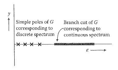
Thus, we have found the formal solution of Equation Eq. 14.2. Let us look at this solution more carefully. Note that \(H\) is a Hermitian operator, which implies that all of its eigenvalues \(\varepsilon_i\) are real. This further implies that for \(y=\operatorname{Im}z\ne0\), \(G(\vec r,\vec r',z)\) is an analytic function of \(z\) in the entire complex plane. If the spectrum of \(H\) is discrete, \(G(\vec r,\vec r',z)\) has poles at \(z=\varepsilon_i\). Since \(\varepsilon_i\) is real, these poles will lie on the real \(z\)-axis. This implies that if we know the poles of Green’s function, we can find discrete eigenvalues of \(H\). If spectrum of \(H\) is continuous, \(G(\vec r,\vec r',z)\) is not defined over that portion of the real \(z\)-axis corresponding to the continuous spectrum of \(H\). If the eigenstates of \(H\) are extended, this produces a branch cut on the real \(z\)-axis as shown in Fig. 14.1. This means that side limits of \(G(\vec r,\vec r',\varepsilon+iy)\) as \(y\to0^+\) exist but are different from each other.
Let us define these side limits as follows:
\[ G^+(\vec r,\vec r',\varepsilon)=\lim_{y\to0^+}G(\vec r,\vec r',\varepsilon+iy) \tag{14.17}\]
\[ G^-(\vec r,\vec r',\varepsilon)=\lim_{y\to0^+}G(\vec r,\vec r',\varepsilon-iy) \tag{14.18}\]
where \(\varepsilon\) is in the continuous part of the spectrum. To show that these limits exist and that there is a discontinuity in \(G(\vec r,\vec r',z)\) as one crosses the branch cut, we shall use the following identity:
\[ \lim_{y\to0}\frac{1}{\varepsilon\pm iy-a}=P\frac{1}{\varepsilon-a}\mp i\pi\delta(\varepsilon-a) \tag{14.19}\]
where \(P\) stands for the principal value, the meaning of which will be clear in the proof given below.
To prove Equation Eq. 14.19, let us consider the integral
\[ \lim_{y\to0}\int\frac{f(\varepsilon)}{\varepsilon+iy-a}d\varepsilon \tag{14.20}\]
where \(f(\varepsilon)\) is a smooth function without any singularities.
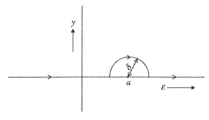
We see that in evaluating Equation Eq. 14.20, the problem arises close to \(\varepsilon=a\), as there is a pole at \(\varepsilon=a\). This means that except for a small interval from \(a-\delta\) to \(a+\delta\), where \(\delta\) is small, we can integrate Equation Eq. 14.20 by putting \(y=0\) but near \(\varepsilon=a\) we have to be careful. Thus, near \(\varepsilon=a\), we slightly deform the path of integration as shown in Fig. 14.2.
The integral over the straight line which avoids the range \(a-\delta\) to \(a+\delta\) is called the principal value, denoted by sign \(P\). To find the contribution from the semicircular path, let us write
\[ z=a+\delta\exp(i\theta) \]
The semicircle is infinitesimally small (as \(\delta\) is very small) but gives a finite contribution to the integral. This is equal to
\[ \int_{\mathrm{semicircle}}\frac{f(z)}{z-a}dz=\int_\pi^0\frac{f(a)}{\delta e^{i\theta}}i\delta e^{i\theta}d\theta=-i\pi f(a) \]
Thus, the integral in Equation Eq. 14.20 can be written as
\[ \lim_{y\to0}\int\frac{f(\varepsilon)}{\varepsilon+iy-a}d\varepsilon=P\int\frac{f(\varepsilon)}{\varepsilon-a}d\varepsilon-i\pi f(a) \tag{14.21}\]
or we can write it symbolically as
\[ \lim_{y\to0}\frac{1}{\varepsilon+iy-a}=P\frac{1}{\varepsilon-a}-i\pi\delta(\varepsilon-a) \tag{14.22}\]
We can see that if we consider \(\varepsilon-iy-a\) instead of \(\varepsilon+iy-a\) in Equation Eq. 14.22, the only difference we will get is \(+\mathrm{ve}\) sign in the last term, which proves identity Eq. 14.19.
Let us apply identity Eq. 14.22 to evaluate Equations Eq. 14.17 and Eq. 14.18. Thus, from Equations Eq. 14.16 and Eq. 14.17
\[ G^+(\vec r,\vec r',\varepsilon)=\lim_{y\to0}\sum_i\frac{\psi_i(\vec r)\psi_i^*(\vec r')}{\varepsilon+iy-\varepsilon_i} \tag{14.23}\]
\[ G^+(\vec r,\vec r',\varepsilon)=P\sum_i\frac{\psi_i(\vec r)\psi_i^*(\vec r')}{\varepsilon-\varepsilon_i}-i\pi\sum_i\delta(\varepsilon-\varepsilon_i)\psi_i(\vec r)\psi_i^*(\vec r') \tag{14.24}\]
Here, summation over \(i\) implies summation over discrete as well as continuous portions of the spectrum. Let us put \(\vec r'=\vec r\) in Equation Eq. 14.24. Then,
\[ G^+(\vec r,\vec r,\varepsilon)=P\sum_i\frac{|\psi_i(\vec r)|^2}{\varepsilon-\varepsilon_i}-i\pi\sum_i\delta(\varepsilon-\varepsilon_i)|\psi_i(\vec r)|^2 \tag{14.25}\]
We see that the first term is real while the last term is imaginary. Taking the imaginary part and integrating it over \(\vec r\), we get
\[ \begin{aligned} \int\operatorname{Im}G^+(\vec r,\vec r,\varepsilon)d^3r &=-\pi\sum_i\delta(\varepsilon-\varepsilon_i)\int|\psi_i(\vec r)|^2d^3r\\ &=-\pi\sum_i\delta(\varepsilon-\varepsilon_i)=-\pi N\rho(\varepsilon) \end{aligned} \tag{14.26}\]
where \(\rho(\varepsilon)=(1/N)\sum_i\delta(\varepsilon-\varepsilon_i)\) is the DOS and \(N\) is the number of cells in the solid. Thus,
\[ \rho(\varepsilon)=-\frac{1}{\pi N}\int\operatorname{Im}G^+(\vec r,\vec r,\varepsilon)d^3r \tag{14.27}\]
This is an important result and is frequently used to calculate the DOS if Green’s function is known. Note that the integration in Equation Eq. 14.27 is overall the volume of the solid. However, in periodic solids, the integration can be limited to one unit cell as each unit cell, contributes the same due to the periodicity. In that case, the factor of \(N\) in Equation Eq. 14.27 cancels out. This result can also be written as
\[ \rho(\varepsilon)=-\frac{1}{\pi N}\operatorname{Im}\operatorname{Tr}G^+(\varepsilon) \tag{14.28}\]
where \(\operatorname{Tr}\) stands for trace. Similarly, if we take an imaginary part of \(G^+(\vec r,\vec r,\varepsilon)\) in Equation Eq. 14.25 and integrate over energy \(\varepsilon\) we get
\[ \begin{aligned} \int_{-\infty}^{\varepsilon_F}\operatorname{Im}G^+(\vec r,\vec r,\varepsilon)d\varepsilon &=-\pi\sum_i|\psi_i(\vec r)|^2\int_{-\infty}^{\varepsilon_F}\delta(\varepsilon-\varepsilon_i)d\varepsilon\\ &=-\pi\sum_{i\ \mathrm{occupied}}|\psi_i(\vec r)|^2=-\pi n(\vec r) \end{aligned} \]
or
\[ n(\vec r)=-\frac{1}{\pi}\int_{-\infty}^{\varepsilon_F}\operatorname{Im}G^+(\vec r,\vec r,\varepsilon)d\varepsilon \tag{14.29}\]
Here, \(n(\vec r)\) is the electron density and we have assumed that all the levels up to the Fermi energy, \(\varepsilon_F\), are filled (\(T=0\) K case). Equation Eq. 14.29 is another important result that relates electron density to Green’s function. Another useful result can be derived as follows:
\[ \begin{aligned} G(\vec r,\vec r',z)&=\sum_i\frac{\psi_i(\vec r)\psi_i^*(\vec r')}{z-\varepsilon_i}\\ &=\sum_i\int\delta(\varepsilon-\varepsilon_i)\frac{\psi_i(\vec r)\psi_i^*(\vec r')}{z-\varepsilon}d\varepsilon\\ &=\int\frac{1}{z-\varepsilon}\sum_i\delta(\varepsilon-\varepsilon_i)\psi_i(\vec r)\psi_i^*(\vec r')d\varepsilon\\ &=-\frac{1}{\pi}\int\frac{\operatorname{Im}G^+(\vec r,\vec r',\varepsilon)}{z-\varepsilon}d\varepsilon \end{aligned} \]
By taking trace of both sides, we get
\[ \operatorname{Tr}G(z)=-\frac{1}{\pi}\int\frac{\operatorname{Im}\operatorname{Tr}G^+(\varepsilon)}{z-\varepsilon}d\varepsilon=\int\frac{N\rho(\varepsilon)}{z-\varepsilon}d\varepsilon \tag{14.30}\]
where we have used Equation Eq. 14.28.
Let us now get back to Equation Eq. 14.24. If we now evaluate \(G(\vec r,\vec r',\varepsilon)\) by replacing \(\varepsilon+iy\) to \(\varepsilon-iy\) in Equation Eq. 14.23, the only change we will get in Equation Eq. 14.24 will be the \(+\) sign of the second term. Thus, in general, we get two different limits of Green’s function \(G(\vec r,\vec r',\varepsilon+iy)\) depending on whether we go from below or above in the complex energy plane. If the spectrum is discrete and \(\varepsilon\ne\varepsilon_i\), that is, we avoid the poles, then these limits are the same. However, if \(\varepsilon\) lies in the continuous spectrum, there is no way of crossing the real axis without avoiding this discontinuity. As we have seen above, this discontinuity is related to the DOS.
From Equation Eq. 14.16, we see that
\[ G^+(\vec r,\vec r',z)=G^-(\vec r',\vec r,z^*) \tag{14.31}\]
or in matrix form, we can write
\[ G^\dagger(z)=G(z^*) \tag{14.32}\]
where \(\dagger\) denotes the Hermitian conjugate. Green’s function \(G(z)\) satisfies the criteria of the Herglotz function. A function \(F(z)\) is Herglotz if it satisfies the following properties.
\(F(z)\) is an analytic function of \(z\) in the entire complex plane except at the real axis, that is, for \(\operatorname{Im}z\ne0\). Its spectrum is bounded and \(F(z)\) behaves as \(1/z\) as \(z\to\pm\infty\).
\[ F^*(z)=F(z^*) \tag{14.33}\]
- \(\operatorname{Im}F(z)<0\) for \(\operatorname{Im}z>0\).
Clearly \(G(z)\) satisfies all these properties.
Now, we shall show that the formal solution of the following inhomogeneous differential equation can be written in terms of Green’s function:
\[ (z-H(\vec r))\psi(\vec r)=f(\vec r) \tag{14.34}\]
We know that \(G(\vec r,\vec r',z)\) satisfies the equation
\[ (z-H(\vec r))G(\vec r,\vec r',z)=\delta(\vec r-\vec r') \tag{14.35}\]
Then \(\psi(\vec r)\) can be written as
\[ \psi(\vec r)=\phi(\vec r)+\int G(\vec r,\vec r',z)f(\vec r')d^3r' \qquad \text{for } z\ne\varepsilon_i \tag{14.36}\]
where \(\phi(\vec r)\) is the solution of the homogeneous equation (i.e., without \(f(\vec r)\) in Equation Eq. 14.34) at energy \(\varepsilon\). Equation Eq. 14.36 is indeed a solution of Equation Eq. 14.34, which can be checked by substituting for \(\psi(\vec r)\) into Equation Eq. 14.34 and then using Equation Eq. 14.35. Note that both \(\phi(\vec r)\) and \(\psi(\vec r)\) should satisfy the same boundary conditions. We see that Green’s function provides a method to solve an inhomogeneous differential equation like Equation Eq. 14.34, provided we know Green’s function.
In summary, we have shown that Green’s function \(G(\vec r,\vec r',z)\) is an analytic function in the whole complex plane except on the real axis. Its poles give the discrete eigenvalues. Its branch cut along the real axis corresponds to the continuous spectrum of \(H\) and the discontinuity in \(G(\vec r,\vec r',z)\) across this branch cut is related to the DOS and the electron density.
14.3 Perturbation Theory Using Green’s Function
One advantage of using Green’s function is that it is relatively easier to handle perturbations. Another advantage is that there is no need to assume the perturbation to be small as is the case with usual perturbation theory. This makes it a much more powerful tool.
Let us divide our one electron Hamiltonian \(H\) into two parts, unperturbed Hamiltonian \(H_0\) and a perturbation \(H_1\),
\[ H=H_0+H_1 \tag{14.37}\]
We assume that the eigenvalues \(\varepsilon_i^0\) and the eigenfunction \(|\psi_i^0\rangle\) of \(H_0\) are known so that Green’s function \(G_0(z)\)
\[ G_0(z)=(z-H_0)^{-1}=\sum_i\frac{|\psi_i^0\rangle\langle\psi_i^0|}{z-\varepsilon_i^0} \tag{14.38}\]
is also known. Our aim is to find Green’s function \(G(z)\) for the Hamiltonian \(H\), given by
\[ \begin{aligned} G(z)&=(z-H)^{-1}\\ &=(z-H_0-H_1)^{-1}\\ &=[(z-H_0)(1-(z-H_0)^{-1}H_1)]^{-1} \end{aligned} \tag{14.39}\]
\[ \begin{aligned} &=[G_0^{-1}(1-G_0H_1)]^{-1}\\ &=(1-G_0H_1)^{-1}G_0 \end{aligned} \tag{14.40}\]
or
\[ \begin{aligned} (1-G_0H_1)G&=G_0\\ G&=G_0+G_0H_1G \end{aligned} \tag{14.41}\]
Equation Eq. 14.41 is known as Dyson’s equation. This can be rewritten as
\[ \begin{aligned} G&=G_0+G_0H_1(G_0+G_0H_1G)\\ &=G_0+G_0H_1G_0+G_0H_1G_0H_1G_0+\cdots\\ &=G_0+G_0(H_1+H_1G_0H_1+\cdots)G_0 \end{aligned} \tag{14.42}\]
\[ G=G_0+G_0TG_0 \tag{14.43}\]
where we have introduced an operator \(T\), which is called \(t\)-matrix and is given by
\[ \begin{aligned} T&=H_1+H_1G_0H_1+\cdots \end{aligned} \tag{14.44}\]
\[ \begin{aligned} &=H_1+H_1G_0(H_1+H_1G_0H_1+\cdots)\\ &=H_1+H_1G_0T \end{aligned} \tag{14.45}\]
\[ \begin{aligned} &=H_1+(H_1+H_1G_0H_1+\cdots)G_0H_1\\ &=H_1+TG_0H_1 \end{aligned} \tag{14.46}\]
It is clear from Equation Eq. 14.43 that if \(T\) is known, \(G\) can be found. Equation Eq. 14.44 can be rewritten as
\[ \begin{aligned} T&=H_1[1+G_0H_1+G_0H_1G_0H_1+\cdots]\\ &=H_1[G_0+G_0H_1G_0+\cdots]G_0^{-1}\\ &=H_1GG_0^{-1}=G_0^{-1}GH_1 \end{aligned} \tag{14.47}\]
\[ =H_1G(z-H_0) \tag{14.48}\]
where we have used Equation Eq. 14.38. From Equation Eq. 14.48, it is clear that \(T(z)\) will have analytic properties similar to \(G(z)\), that is, it will be analytic in the whole complex \(z\)-plane except on the real axis. Various techniques such as diagrammatic techniques have been used to evaluate \(T(z)\), but we shall not discuss them here.
The above equations are written in matrix form in Hilbert space but can be easily written in real or \(k\)-space. For example, Equation Eq. 14.41 can be written in real space as
\[ G(\vec r,\vec r',z)=G_0(\vec r,\vec r',z)+\iint G_0(\vec r,\vec r_1,z)H_1(\vec r_1,\vec r_2)G(\vec r_2,\vec r',z)d^3r_1d^3r_2 \tag{14.49}\]
or in \(k\)-space
\[ G(\vec k,\vec k',z)=G_0(\vec k,\vec k',z)+\sum_{\vec k_1\vec k_2}G_0(\vec k,\vec k_1,z)H_1(\vec k_1,\vec k_2)G(\vec k_2,\vec k',z) \tag{14.50}\]
We now discuss how the eigenstates \(|\psi\rangle\) associated with \(H\) can be found. Let \(|\phi\rangle\) be the eigenstates of \(H_0\) that is
\[ (\varepsilon-H_0)|\phi\rangle=0 \tag{14.51}\]
and
\[ (\varepsilon-H)|\psi\rangle=0 \tag{14.52}\]
or
\[ (\varepsilon-H_0-H_1)|\psi\rangle=0 \]
or
\[ (\varepsilon-H_0)|\psi\rangle=H_1|\psi\rangle \tag{14.53}\]
Thus, \(|\psi\rangle\) can be written as
\[ |\psi\rangle=|\phi\rangle+G_0(\varepsilon)H_1|\psi\rangle \tag{14.54}\]
This can be checked by substituting Equation Eq. 14.54 into Equation Eq. 14.53. If \(\varepsilon\) does not belong to the spectrum of \(H_0\), then
\[ |\psi\rangle=G_0(\varepsilon)H_1|\psi\rangle \tag{14.55}\]
or
\[ \psi(\vec r)=\int G_0(\vec r,\vec r',\varepsilon)H_1(\vec r')\psi(\vec r')d^3r' \tag{14.56}\]
Equation Eq. 14.56 can be used to find eigenfunctions corresponding to the discrete spectrum assuming that none of the discrete eigenvalues of \(H\) and \(H_0\) coincide. If \(H_0\) is taken to be the free electron Hamiltonian, it has no discrete spectrum and we can use Equation Eq. 14.56 without any problem to find \(\psi(\vec r)\) corresponding to the discrete spectrum of \(H\). If \(\varepsilon\) belongs to the continuous part of the spectrum, then the limiting procedure as discussed before has to be used, that is, we have to use \(G_0^\pm(\varepsilon)\) in Equation Eq. 14.54
\[ |\psi^\pm\rangle=|\phi\rangle+G_0^\pm(\varepsilon)H_1|\psi^\pm\rangle \tag{14.57}\]
or
\[ \psi^\pm(\vec r)=\phi(\vec r)+\iint G_0^\pm(\vec r,\vec r',\varepsilon)H_1(\vec r',\vec r'')\psi^\pm(\vec r'')d^3r'd^3r'' \tag{14.58}\]
Generally \(H_1(\vec r',\vec r'')=\delta(\vec r'-\vec r'')v(\vec r')\), thus
\[ \psi^\pm(\vec r)=\phi(\vec r)+\int G_0^\pm(\vec r,\vec r',\varepsilon)v(\vec r')\psi^\pm(\vec r')d^3r' \tag{14.59}\]
Equation Eq. 14.58 or Equation Eq. 14.59 is called the Lippman-Schwinger equation. Note that if \(\phi(\vec r)\) does not satisfy the same boundary condition as \(\psi^\pm(\vec r)\), it should be dropped in these equations.
Let us now express Equation Eq. 14.57 in terms of \(T\). This can be done by substituting for \(|\psi^\pm\rangle\) on the right-hand side of Equation Eq. 14.57, that is
\[ \begin{aligned} |\psi^\pm\rangle&=|\phi\rangle+G_0^\pm(\varepsilon)H_1|\phi\rangle+G_0^\pm(\varepsilon)H_1G_0^\pm(\varepsilon)H_1|\phi\rangle+\cdots\\ &=|\phi\rangle+G_0^\pm(H_1+H_1G_0H_1+\cdots)|\phi\rangle\\ &=|\phi\rangle+G_0^\pm T^\pm|\phi\rangle \end{aligned} \tag{14.60}\]
Comparing Equations Eq. 14.57 and Eq. 14.60, we get
\[ H_1|\psi^\pm\rangle=T^\pm|\phi\rangle \tag{14.61}\]
Equation Eq. 14.47 can also be written as
\[ T=G_0^{-1}GH_1 \]
or
\[ G_0T=GH_1 \]
Substituting this into Equation Eq. 14.60 we get,
\[ |\psi^\pm\rangle=|\phi\rangle+G^\pm H_1|\phi\rangle \tag{14.62}\]
Equations Eq. 14.60 and Eq. 14.62 are sometimes very useful as these express \(|\psi^\pm\rangle\) in terms of \(|\phi\rangle\) and not in terms of \(|\psi^\pm\rangle\) as is the case with Equation Eq. 14.57.
14.4 Free Electron Green’s Function in Three Dimensions
As an example, we shall find Green’s function for a free electron gas in three dimensions (3D). For simplicity, we shall use the atomic units (a.u.) in this section (see Appendix C).
For the free electron gas, the Hamiltonian, its eigenvalues, and eigenfunctions are given by
\[ H(\vec r)=-\frac{\hbar^2}{2m_e}\nabla^2=-\frac{1}{2}\nabla^2 \qquad \text{(in a.u.)} \tag{14.63}\]
\[ \varepsilon_k=\frac{\hbar^2k^2}{2m_e}=\frac{k^2}{2} \qquad \text{(in a.u.)} \tag{14.64}\]
\[ \langle \vec r|\vec k\rangle=\frac{1}{\sqrt{\Omega}}e^{i\vec k\cdot\vec r} \tag{14.65}\]
Green’s function satisfies the equation
\[ \left(z+\frac{\nabla^2}{2}\right)G(\vec r,\vec r',z)=\delta(\vec r-\vec r') \tag{14.66}\]
Using Equation Eq. 14.14, the solution of Equation Eq. 14.66 can be written as
\[ G(\vec r,\vec r',z)=\sum_{\vec k}\frac{\langle\vec r|\vec k\rangle\langle\vec k|\vec r'\rangle}{z-k^2/2}=\int\frac{e^{i\vec k\cdot(\vec r-\vec r')}}{z-k^2/2}\frac{d^3k}{(2\pi)^3} \tag{14.67}\]
To evaluate the integral in Equation Eq. 14.67, let us write
\[ \vec d=(\vec r-\vec r') \]
Also we choose spherical polar coordinates such that \(k_z\) axis coincides with \(\vec d\). Thus,
\[ e^{i\vec k\cdot(\vec r-\vec r')}=e^{i\vec k\cdot\vec d}=e^{ikd\cos\theta} \]
Therefore, Equation Eq. 14.67 can be written as
\[ \begin{aligned} G(\vec r,\vec r',z)&=\int\frac{e^{ikd\cos\theta}}{z-k^2/2}\frac{d^3k}{(2\pi)^3}\\ &=\int\frac{2\pi k^2dk}{z-k^2/2}\frac{1}{(2\pi)^3}\int_0^\pi e^{ikd\cos\theta}\sin\theta d\theta\\ &=\frac{1}{4\pi^2}\int_0^\infty\frac{k^2dk}{z-k^2/2}\left[-\frac{e^{ikd\cos\theta}}{ikd}\right]_0^\pi\\ &=\frac{1}{4\pi^2id}\int_0^\infty\frac{k(e^{ikd}-e^{-ikd})}{z-k^2/2}dk\\ &=\frac{1}{4\pi^2id}\int_{-\infty}^{\infty}\frac{ke^{ikd}}{z-k^2/2}dk \end{aligned} \tag{14.68}\]
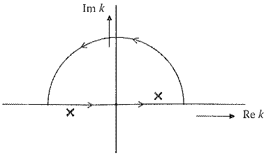
The integral in Equation Eq. 14.68 can be easily evaluated in a complex plane. We first note that the integrand has poles at
\[ k^\pm=\pm\sqrt{2z} \tag{14.69}\]
One of these poles will have positive imaginary part unless \(z\) is a real and positive number. Thus, the integration in Equation Eq. 14.68 can be done by closing the path by an infinite semicircle in the upper half-plane as shown in Fig. 14.3 and then using the residue theorem.
Here, we are interested in finding \(G^\pm(\vec r,\vec r',\varepsilon)\). Let us first calculate \(G^+(\vec r,\vec r',\varepsilon)\) and write \(z=\varepsilon+iy\) where \(y\to0\). Thus,
\[ \begin{aligned} k^\pm&=\pm\sqrt{2(\varepsilon+iy)}\\ &=\pm\sqrt{2\varepsilon}\left(1+\frac{iy}{\varepsilon}\right)^{1/2}\\ &=\pm\sqrt{2\varepsilon}\left(1+\frac{iy}{2\varepsilon}\right) \end{aligned} \tag{14.70}\]
Thus, the integral \(I\) in Equation Eq. 14.68 is
\[ \begin{aligned} I&=\lim_{k\to k^+}2\pi i\frac{k e^{ikd}}{(\sqrt{2z}-k)(\sqrt{2z}+k)}(k-k^+)\\ &=-2\pi i e^{i\sqrt{2\varepsilon}d} \end{aligned} \]
Thus,
\[ G^+(\vec r,\vec r',\varepsilon)=-\frac{1}{4\pi^2id}2\pi i e^{i\sqrt{2\varepsilon}d}=-\frac{1}{2\pi}\frac{e^{i\sqrt{2\varepsilon}|\vec r-\vec r'|}}{|\vec r-\vec r'|}\qquad \varepsilon>0 \tag{14.71}\]
To calculate \(G^-(\vec r,\vec r',\varepsilon)\), we will have to replace \(z\) by \(\varepsilon-iy\) and then take \(y\to0\) limit. Now the pole lying in the upper half of the complex plane is \(k^-=-\sqrt{2\varepsilon}(1-iy/(2\varepsilon))\). This will give
\[ G^-(\vec r,\vec r',\varepsilon)=-\frac{1}{2\pi}\frac{e^{-i\sqrt{2\varepsilon}|\vec r-\vec r'|}}{|\vec r-\vec r'|}\qquad \varepsilon>0 \tag{14.72}\]
Note that for \(\varepsilon>0\), \(G^+\) and \(G^-\) have discontinuity as expected. For \(\varepsilon<0\), there is no singularity in the integrand in Equation Eq. 14.68 on the real axis. Now, the poles are on the imaginary axis,
\[ k^\pm=\pm\sqrt{2(-|\varepsilon|)}^{1/2}=\pm i\sqrt{2|\varepsilon|} \]
Green’s function, then, is given by
\[ G(\vec r,\vec r',\varepsilon)=-\frac{1}{2\pi}\frac{e^{-\sqrt{2|\varepsilon|}|\vec r-\vec r'|}}{|\vec r-\vec r'|}\qquad \varepsilon<0 \tag{14.73}\]
From Equation Eq. 14.71
\[ \operatorname{Im}G^+(\vec r,\vec r',\varepsilon)=-\frac{1}{2\pi}\frac{\sin(\sqrt{2\varepsilon}|\vec r-\vec r'|)}{|\vec r-\vec r'|} \]
\[ \lim_{\vec r'\to\vec r}\operatorname{Im}G^+(\vec r,\vec r',\varepsilon)=-\frac{\sqrt{2\varepsilon}}{2\pi} \]
The DOS \(\rho(\varepsilon)\) is, thus, given by
\[ \rho(\varepsilon)=-\frac{1}{\pi N}\int\operatorname{Im}G^+(\vec r,\vec r,\varepsilon)d^3r=\frac{\Omega}{2N\pi^2}\sqrt{2\varepsilon} \tag{14.74}\]
which goes as \(\varepsilon^{1/2}\) as expected.
14.5 Korringa-Kohn-Rostoker (KKR) Method
The KKR method was first developed by Korringa (1947) and then by Kohn and Rostoker (1954) to calculate the energy bands in solids and is known as the KKR method. It can be generalized to disordered alloys as we shall see in the next chapter. The KKR method is also known as the Green’s function method as it is formulated in terms of Green’s function. The details of the method are quite involved so here I shall only give a brief outline.
Let us consider an electron moving in a periodic potential \(v(\vec r)\). Our aim is to find energy bands, which are obtained by solving the Kohn-Sham equation,
\[ \left(-\frac{\hbar^2}{2m_e}\nabla^2+v(\vec r)\right)\psi_i(\vec r)=\varepsilon_i\psi_i(\vec r) \]
or in atomic units
\[ \left(\varepsilon_i+\frac{\nabla^2}{2}\right)\psi_i(\vec r)=v(\vec r)\psi_i(\vec r) \tag{14.75}\]
We already know the solution of Equation Eq. 14.75 without \(v(\vec r)\), which are plane waves given by Equation Eq. 14.65 and the corresponding Green’s function Eq. 14.71. We can use Equation Eq. 14.59 to write the solution of Equation Eq. 14.75 as
\[ \psi_i(\vec r)=\int G_0^+(\vec r,\vec r',\varepsilon_i)v(\vec r')\psi_i(\vec r')d^3r' \tag{14.76}\]
There are two points that are worth noting regarding Equation Eq. 14.76. First, we have chosen \(G_0^+\) to build up our solution, which is the normal practice in the literature, but the whole analysis can be carried out using \(G_0^-\) as well. Second, we have not added in Equation Eq. 14.76, the solution of homogenous equation, which is a plane wave. This is related to the boundary condition. Since \(v(\vec r)\) is periodic, \(\psi_i(\vec r)\) satisfies Bloch’s theorem
\[ \psi_i(\vec r+\vec R_j)=e^{i\vec k\cdot\vec R_j}\psi_i(\vec r) \tag{14.77}\]
where \(\vec R_j\) is a lattice vector. The solution of Equation Eq. 14.75 with \(v(\vec r)=0\) is
\[ \phi=\frac{1}{\sqrt{\Omega}}e^{i\vec k'\cdot\vec r} \tag{14.78}\]
where
\[ k'=\sqrt{2\varepsilon_i} \tag{14.79}\]
From this, it is clear that in general \(\vec k'\ne\vec k\). Thus, \(\psi_i(\vec r)\) and \(\phi(\vec r)\) cannot satisfy Bloch’s theorem with the same \(\vec k\) and the only way \(\psi_i(\vec r)\) can satisfy Bloch’s theorem is to drop \(\phi(\vec r)\).
The periodic potential \(v(\vec r)\) can be written as
\[ v(\vec r)=\sum_j v_a(\vec r-\vec R_j) \tag{14.80}\]
where \(v_a(\vec r)\) is the contribution from each atom. Here, we are assuming that there is only one atom per primitive cell. The potential \(v_a(\vec r)\) is assumed to be of the muffin-tin form, that is
\[ v_a(\vec r)= \begin{cases} v_a(r), & \text{if } r\le r_m,\\ 0, & \text{if } r>r_m. \end{cases} \tag{14.81}\]
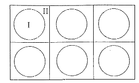
That is, the potential \(v_a(\vec r)\) is assumed to be spherically symmetric within a radius, \(r_m\), called the muffin-tin radius, and is assumed to be zero in the remaining part of the primitive cell. The muffin-tin potentials are nonoverlapping potentials as shown schematically in Fig. 14.4 for a two-dimensional solid. The solid is assumed to have a square lattice. The figure shows few unit cells (Wigner-Seitz unit cell) and each cell is divided into two regions, I and II. Inside the circles (region I), the potential is attractive and deep (see Fig. 13.3) but outside the circle (region II) it is flat. We see that Fig. 14.4 looks like a muffin-tin and thus such a potential is called a muffin-tin potential. This kind of potential was first proposed by Slater while developing the APW method (see Section Section 14.7).
Substituting Equation Eq. 14.71 for \(G_0^+\) and Equation Eq. 14.81 for \(v(\vec r)\) into Equation Eq. 14.76, we get
\[ \psi_{\vec k}(\vec r)=-\frac{1}{2\pi}\sum_j\int\frac{e^{i\kappa|\vec r-\vec r'|}}{|\vec r-\vec r'|}v_a(\vec r'-\vec R_j)\psi_{\vec k}(\vec r')d^3r' \tag{14.82}\]
where
\[ \kappa=\sqrt{2\varepsilon} \tag{14.83}\]
Replacing \(\vec r'\) by \(\vec r'+\vec R_j\) and using Equation Eq. 14.77, we get
\[ \begin{aligned} \psi_{\vec k}(\vec r)&=-\frac{1}{2\pi}\sum_j\int\frac{e^{i\kappa|\vec r-\vec r'-\vec R_j|}}{|\vec r-\vec r'-\vec R_j|}v_a(\vec r')e^{i\vec k\cdot\vec R_j}\psi_{\vec k}(\vec r')d^3r'\\ &=-\frac{1}{2\pi}\int g(\vec r,\vec r',\kappa,\vec k)v_a(\vec r')\psi_{\vec k}(\vec r')d^3r' \end{aligned} \tag{14.84}\]
where
\[ g(\vec r,\vec r',\kappa,\vec k)=\sum_j\frac{e^{i\kappa|\vec r-\vec r'-\vec R_j|}}{|\vec r-\vec r'-\vec R_j|}e^{i\vec k\cdot\vec R_j} \tag{14.85}\]
and is called structural Green’s function as it depends only on the structure of the lattice and not on the potential. Since \(v_a(\vec r')\) is zero outside the radius \(r_m\), the integration in Equation Eq. 14.84 is limited only over a single muffin-tin sphere.
Now a functional \(\Lambda\) is constructed, which upon variation gives Equation Eq. 14.84. This can easily be seen to be
\[ \Lambda=\int\psi_{\vec k}^*(\vec r)v_a(\vec r)\psi_{\vec k}(\vec r)d^3r+\frac{1}{2\pi}\iint\psi_{\vec k}^*(\vec r)v_a(\vec r)g(\vec r,\vec r',\kappa,\vec k)v_a(\vec r')\psi_{\vec k}(\vec r')d^3rd^3r' \tag{14.86}\]
This can be seen by taking the functional derivative \(\delta\Lambda/\delta\psi_{\vec k}^*(\vec r)\) and setting it to be zero. Note that in addition to \(\psi_{\vec k}(\vec r)\), \(v_a(\vec r)\) was also introduced in Equation Eq. 14.86. This has the advantage that all the integrals in Equation Eq. 14.86 are over muffin-tin spheres. These integrals can further be simplified by using Green’s identity, which reduces them to surface integrals over the spheres.
The use of muffin-tin potential has more advantages. As it is spherically symmetric, we can choose a trial function of the following form inside each cell:
\[ \psi_{\vec k}(\vec r)=\sum_{\ell m}C_{\ell m}\phi_\ell(r)Y_{\ell m}(\theta,\varphi)=\sum_LC_L\phi_\ell(r)Y_L(\theta,\varphi) \tag{14.87}\]
where \(\phi_\ell(r)\) is the solution of the radial Schrodinger equation for \(v_a(r)\) and \(Y_{\ell m}(\theta,\varphi)\) are the spherical harmonics. In Equation Eq. 14.87, we have used a composite index \(L=(\ell,m)\). The substitution of Equation Eq. 14.87 into Equation Eq. 14.86 leads to a function
\[ \Lambda=\sum_{LL'}\mathcal{A}_{LL'}C_LC_{L'}^* \tag{14.88}\]
where \(\mathcal{A}_{LL'}\) are coefficients and here we shall not discuss how to evaluate them. For details, the paper by Kohn and Rostoker (1954) should be consulted. However, the final form of \(\mathcal{A}_{LL'}\) is quite interesting, therefore, I shall just quote the final result, which is
\[ \mathcal{A}_{LL'}=A_{LL'}+\kappa\delta_{LL'}\cot\delta_\ell \tag{14.89}\]
Here, the coefficients \(A_{LL'}\) depend on \(\vec k,\kappa\) and the structure of the solid and are called KKR structure constants. In Equation Eq. 14.89, \(\delta_\ell\) are phase shifts which depend only on the potential (see Chapter Section 13.1). Thus, the form of Equation Eq. 14.89 is particularly suited for efficient computation. For the same structure, one need not calculate \(A_{LL'}\) again and again.
The variational functional \(\Lambda\) in Equation Eq. 14.88 has to be minimized with respect to \(C_L^*\), and this leads to a set of linear algebraic equations in \(C_L\), that is
\[ \sum_{L'}\mathcal{A}_{LL'}C_{L'}=0 \tag{14.90}\]
These equations have nontrivial solution only if
\[ \det|\mathcal{A}_{LL'}|=0 \]
or from Equation Eq. 14.89
\[ \det|A_{LL'}+\kappa\delta_{LL'}\cot\delta_\ell|=0 \tag{14.91}\]
This is the KKR secular equation. This determinant is a function of \(\vec k\) and energy \(\varepsilon\), and its roots give the band structure, that is, \(\varepsilon_i\) vs. \(\vec k\). For calculating band structure, one fixes \(\vec k\) and varies \(\varepsilon\) to find the roots of the determinant. In principle, the size of the determinant in Equation Eq. 14.91 is infinite, but in practical calculation, \(\ell_{max}\) is chosen at about 3. This makes the size of the determinant \(16\times16\), which is quite small. Using this method, Moruzzi et al. (1978) have calculated band structures of a large number of elemental solids and were able to explain various trends seen in properties such as bulk modulus, cohesive energy, and Wigner-Seitz radius. This proved to be a turning point that established the density function theory as the foundation on which most electronic structure calculations are based.
The muffin-tin approximation to the potential is the main approximation in the KKR method. It is because of this approximation that the calculation becomes quite simple. For metals, this approximation is particularly good, because the charge density is nearly spherically symmetric in a large region around the atom. But in semiconductors and insulators, the charge density is highly directional and the muffin-tin approximation is not a good approximation for these materials. It turned out to be difficult to extend the scheme for the full potential, although several attempts have been made to develop a KKR-type scheme by using the full-potential rather than muffin-tin potential. Such methods are known as full-potential KKR methods or FP-KKR methods. For details, see for example, the paper by Asato et al. (1999), who have done electronic structure calculations using this method for several metals and semiconductors and have found this method quite satisfactory.
14.6 Linear Muffin-Tin Orbital (LMTO) Method
We saw that the energy eigenvalues \(\varepsilon_i\) in methods like the plane wave expansions method were obtained by solving an equation like
\[ \det\left|\left(\varepsilon_{\vec k-\vec G}^0-\varepsilon_{\vec k}\right)\delta_{\vec G\vec G'}+v(\vec G'-\vec G)\right|=0 \tag{14.92}\]
Thus by solving this equation, one could get all the eigenvalues \(\varepsilon_i\) in a single diagonalization. In the KKR method, we get the eigenvalues by finding the roots of the equation
\[ \det|A_{LL'}+\kappa\delta_{LL'}\cot\delta_\ell|=0 \tag{14.93}\]
Finding roots of Equation Eq. 14.93 is a much slower process than getting \(\varepsilon_i\) from Equation Eq. 14.92. The roots are found one by one by changing energy while in the plane wave expansion method, one gets all the eigenvalues in one go. If somehow Equation Eq. 14.93 can be cast in the form of Equation Eq. 14.92, the method can become very fast.
The reason why the KKR method is slow is that the basis set is energy dependent in contrast to the plane wave method. The plane waves form an energy-independent basis set, which results in a simpler secular equation like Equation Eq. 14.92. In the LMTO method, by using a suitable approximation, it was possible to cast the secular equation in the form like Equation Eq. 14.92, thus speeding up the calculation.
Andersen (1975) first constructed a muffin-tin orbital (MTO) \(\phi_L(\varepsilon,\vec r)\) for a single muffin-tin potential and then expanded it around reference energy \(\varepsilon_0\) using Taylor’s expansion retaining terms up to linear in energy, that is
\[ \phi_L(\varepsilon,\vec r)=\phi_L(\varepsilon_0,\vec r)+(\varepsilon-\varepsilon_0)\dot\phi_L(\varepsilon_0,\vec r) \tag{14.94}\]
where \(\dot\phi_L\) is the energy derivative of \(\phi_L\) evaluated at \(\varepsilon=\varepsilon_0\). The orbital \(\phi_L\) given by Equation Eq. 14.94 is called an LMTO. Now, the wave function of electron \(\psi_i(\vec r)\) can be expanded in terms of LMTOs as
\[ \psi_i(\vec r)=\sum_{\vec R,L}a_{\vec R L}^i\phi_L(\varepsilon_i,\vec r-\vec R) \tag{14.95}\]
where the sum is over all the lattice vector \(\vec R\) and angular momentum index \(L\). Here, we have assumed one atom per primitive unit cell. This leads to an equation for \(\varepsilon\) as
\[ \det|H_{LL'}(\vec k)-\varepsilon_iO_{LL'}(\vec k)|=0 \tag{14.96}\]
where \(H_{LL'}(\vec k)\) and \(O_{LL'}(\vec k)\) are energy-independent matrix elements. Equation Eq. 14.96 has the same form as Equation Eq. 14.92 and thus gives all the eigenvalues in a single diagonalization and saves enormous computing time. Andersen also gave the tight-binding version of the LMTO known as the TB-LMTO. More recently, a new NMTO method has been presented, which goes beyond the linear approximation and gives more accurate results. For details, we refer to the original papers (Andersen 1975, Andersen and Saha-Dasgupta 2000).
14.7 Augmented Plane Wave (APW) Method
The APW method was given by J.C. Slater (1937), one of the pioneers in the field of electronic structure. We assume that in each cell the potential is of muffin-tin form, that is, it is spherically symmetric within a radius \(r_m\) and zero outside.
\[ \begin{aligned} v(\vec r)&=v(r)\qquad \text{for } r<r_m,\\ &=0\qquad \text{for } r>r_m. \end{aligned} \]
For simplicity, we assume that we have only one atom per unit cell. Pictorially, it is shown in Fig. 14.4 for a square lattice in two dimensions. We can divide the whole space in two parts: region I corresponding to muffin-tin spheres and region II, the interstitial region as indicated in Fig. 14.4. In region II the potential is zero, so the wave function of the electron in this region is likely to be of extended nature, while in region I it is likely to be of more localized character. Thus, if we could construct a basis which is more localized in region I and has extended character like a plane wave in region II, we are likely to have a very small number of basis functions in the expansion of the wave function of the electron. This is the idea behind the APW method.
In region I, the solution of the Schrodinger equation is of the form
\[ \chi(\vec r)=\sum_{\ell m}a_{\ell m}\phi_\ell(\varepsilon,r)Y_{\ell m}(\hat r) \tag{14.97}\]
where \(Y_{\ell m}(\hat r)\) are spherical harmonics for direction \(\hat r\), \(a_{\ell m}\) the expansion coefficients and \(\phi_\ell(\varepsilon,r)\) satisfies the radial equation (in atomic units)
\[ \left[\frac{1}{2}\left(-\frac{d^2}{dr^2}+\frac{\ell(\ell+1)}{r^2}\right)+v(r)\right]\phi_\ell(\varepsilon,r)=\varepsilon\phi_\ell(\varepsilon,r) \tag{14.98}\]
In the interstitial region the potential is zero and the solutions of the Schrodinger equation are plane waves. Therefore, \(\chi(\vec r)\) given by Equation Eq. 14.97 is exactly matched to plane wave \(e^{i\vec k\cdot\vec r}\) at \(r=r_m\). This condition gives \(a_{\ell m}\) as follows.
Suppose \(\vec r\) lies in \(n\)th cell in the interstitial region, we can write
\[ \vec r=\vec r_n+\vec\rho \tag{14.99}\]
where \(\vec\rho\) is measured with respect to the center of the \(n\)th sphere as shown in Fig. 14.5.
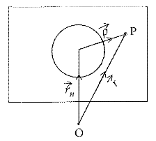
We can write
\[ \begin{aligned} \chi(\vec r)&=e^{i\vec k\cdot\vec r}=e^{i\vec k\cdot(\vec r_n+\vec\rho)}\\ &=e^{i\vec k\cdot\vec r_n}e^{i\vec k\cdot\vec\rho} \end{aligned} \tag{14.100}\]
we can expand \(e^{i\vec k\cdot\vec\rho}\) as
\[ e^{i\vec k\cdot\vec\rho}=4\pi\sum_{\ell m}i^\ell j_\ell(k\rho)Y_{\ell m}(\hat\rho)Y_{\ell m}^*(\hat k) \tag{14.101}\]
so that
\[ e^{i\vec k\cdot\vec r}=4\pi e^{i\vec k\cdot\vec r_n}\sum_{\ell m}i^\ell j_\ell(k\rho)Y_{\ell m}(\hat\rho)Y_{\ell m}^*(\hat k) \tag{14.102}\]
Now matching \(e^{i\vec k\cdot\vec r}\) at the surface of \(n\)th sphere (\(\rho=r_m\)) to Equation Eq. 14.97 gives
\[ a_{\ell m}=4\pi e^{i\vec k\cdot\vec r_n}i^\ell j_\ell(kr_m)Y_{\ell m}^*(\hat k)/\phi_\ell(\varepsilon,r_m) \tag{14.103}\]
Thus, we define an APW as
\[ \chi_{\vec k}(\vec r)= \begin{cases} e^{i\vec k\cdot\vec r}, & \text{outside sphere},\\ 4\pi e^{i\vec k\cdot\vec r_n}\displaystyle\sum_{\ell m}i^\ell j_\ell(kr_m)Y_{\ell m}^*(\hat k)\dfrac{\phi_\ell(\varepsilon,\rho)}{\phi_\ell(\varepsilon,r_m)}Y_{\ell m}(\hat\rho), & \text{inside } n\text{th sphere}. \end{cases} \tag{14.104}\]
Note that \(\chi_{\vec k}(\vec r)\) satisfies Bloch’s theorem.
\[ \chi_{\vec k}(\vec r+\vec R)=e^{i\vec k\cdot\vec R}\chi_{\vec k}(\vec r) \tag{14.105}\]
and is discontinuous in slope at the surface of the muffin-tin sphere. Now, just like in the plane wave or OPW methods, we expand the wave function of the electron in terms of APWs as
\[ \psi_i(\vec r)=\sum_{\vec G}C_{i,\vec k+\vec G}\chi_{\vec k+\vec G}(\vec r) \tag{14.106}\]
where \(C_{i,\vec k+\vec G}\) are unknown coefficients, which are determined by a variational procedure. The wave function Eq. 14.106 is used as a trial wave function and coefficients are adjusted so as to give minimum energy. We shall not go into details of this calculation here and refer to the book by Loucks (1967). The final result has a very interesting form, very much similar to the one we got for the plane wave expansion method,
\[ \sum_{\vec G'}\left\{\left[\frac{1}{2}(\vec k+\vec G)^2-\varepsilon\right]\delta_{\vec G\vec G'}+V_{\vec G\vec G'}(\varepsilon,\vec k)\right\}C_{\vec k+\vec G'}=0 \tag{14.107}\]
where
\[ \begin{aligned} V_{\vec G\vec G'}(\varepsilon,\vec k)&=\frac{4\pi r_m^2}{\Omega_{cell}}\left[\frac{1}{2}|\vec k+\vec G|^2-\varepsilon\right]\frac{j_1(|\vec G-\vec G'|r_m)}{|\vec G-\vec G'|}\\ &\quad+\frac{2\pi r_m^2}{\Omega_{cell}}\sum_\ell(2\ell+1)P_\ell(\cos\theta_{\vec G\vec G'})j_\ell(|\vec k+\vec G'|r_m)j_\ell(|\vec k+\vec G|r_m)\\ &\quad\times\left[\frac{d}{dr}\ln\phi_\ell(\varepsilon,r)-\frac{d}{dr}\ln j_\ell(|\vec k+\vec G|r)\right]_{r=r_m} \end{aligned} \tag{14.108}\]
where \(\theta_{\vec G\vec G'}\) is the angle between \(\vec k+\vec G\) and \(\vec k+\vec G'\). The eigenvalues \(\varepsilon_k\) are obtained by seeking the solution of linear equations in \(C_{\vec k+\vec G}\), which can exist only if the determinant of the coefficients given in curly brackets in Equation Eq. 14.107 vanishes. These coefficients depend on \(\varepsilon\). Thus, one finds the determinant for a certain energy \(\varepsilon\) and then varies it until the root is found as in the KKR method. By repeating this procedure for each \(\vec k\), one can find the band structure \(\varepsilon\) vs. \(\vec k\).
14.8 Linear Augmented Plane Wave (LAPW) Method
One big disadvantage of the APW method is that the basis functions are energy dependent. Thus, the energy bands cannot be determined by a single diagonalization. As we saw above that to find \(\varepsilon_i\), it is necessary to find the secular determinant as a function of \(\varepsilon\) and then find its roots. This is computationally very demanding and a nonlinear procedure to find \(\varepsilon_i\). What we would like is to obtain all eigenvalues at one \(\vec k\) by a single diagonalization as is the case in the plane wave method, where the basis functions are energy independent. In such cases, we have linear equations for eigenvalues. In the LAPW method, this is achieved by defining basis functions as the linear combination of radial function \(\phi_\ell(\varepsilon_0,r)\) and its energy derivative \(\dot\phi_\ell(\varepsilon_0,r)\) evaluated at chosen fixed energy \(\varepsilon_0\). The energy derivative satisfies the equation (in atomic units)
\[ \left[\frac{1}{2}\left(-\frac{d^2}{dr^2}+\frac{\ell(\ell+1)}{r^2}\right)+v(r)-\varepsilon_0\right]\dot\phi_\ell(\varepsilon_0,r)=r\phi_\ell(\varepsilon_0,r) \tag{14.109}\]
where \(\phi_\ell(\varepsilon_0,r)\) satisfies Equation Eq. 14.98, same as in the APW method.
The LAPW basis is defined as
\[ \chi_{\vec k}^{\mathrm{LAPW}}(\vec r)= \begin{cases} e^{i\vec k\cdot\vec r}, & \text{in the interstitial region},\\ \displaystyle\sum_{\ell m}\left[a_{\ell m}\phi_\ell(\varepsilon_0,\rho)+b_{\ell m}\dot\phi_\ell(\varepsilon_0,\rho)\right]Y_{\ell m}(\hat\rho), & \rho<r_m. \end{cases} \]
where \(a_{\ell m}\) and \(b_{\ell m}\) are coefficients, analogous to the APW method and \(\rho\) is measured from the center of the \(n\)th cell (see Fig. 14.5). Thus, the LAPW are just plane waves in the interstitial region but have more variational freedom inside the spheres compared to the APWs. This is because if \(\varepsilon_0\) differs slightly from the band energy, a linear combination will reproduce the APW radial function as
\[ \phi_\ell(\varepsilon,r)=\phi_\ell(\varepsilon_0,r)+(\varepsilon-\varepsilon_0)\dot\phi_\ell(\varepsilon_0,r)+O(\varepsilon-\varepsilon_0)^2 \]
where \(O(\varepsilon-\varepsilon_0)^2\) denotes errors that are quadratic in this energy difference. Thus, the LAPW method introduces error of the order of \((\varepsilon-\varepsilon_0)^2\) in the wavefunction and error of the order of \((\varepsilon-\varepsilon_0)^4\) in the band energy. Because of the high order of this error, the LAPWs form a good basis set over a relatively large energy region, so that all valence bands can be treated with a single set of \(\varepsilon_0\).
The resulting equations have the same form as Equation Eq. 14.107 with the simplification that \(V_{GG'}\) is independent of energy. This is a big advantage because in the LAPW method, one can get all \(\varepsilon_i\) at a \(\vec k\) by a single diagonalization, thus saving much computational cost compared to the APW method. The LAPW method has also been generalized to full potential and is known as the full-potential LAPW (FP-LAPW) method. For details, we refer to the book by Singh and Nordstrom (2006).
14.9 Linear Scaling Methods
The computational effort involved in electronic structure calculations using the methods discussed so far scales at least as \(N^3\), where \(N\) is the number of electrons in the unit cell. This means that if \(N\) is doubled or the cell is doubled, the computational time will increase at least eight times. Thus, treating large unit cells with atoms more than 100 becomes very difficult using these methods. To handle such large systems using the first-principles techniques, several methods, for which computational effort scales linearly with \(N\), have been developed during the last two decades. Such methods are known as linear scaling methods or \(O(N)\) methods. Here, we shall briefly discuss the principle involved to achieve linear scaling. It turns out that linear scaling is not achieved simply by some mathematical trick but involves deep understanding of physics, namely, the concept of locality in quantum mechanics.
The locality in quantum mechanics means that properties of a region comprising of one or a few atoms are mainly dependent on the local environment and weakly influenced by regions which are far from it. For example, semiconductors are often described in terms of covalent bonds which are mainly dependent on the immediate neighborhood. In metals, the total charge density can be obtained within a good accuracy by the superposition of atomic charge densities. Since the atomic charge density decays rapidly with distance, this implies that the charge density in a metal is mainly determined by its local environment. Kohn (1996) describes such quantities which depend mainly on its local environment using the term “nearsightedness.” The “nearsightedness” is a consequence of quantum mechanical destructive interference of electrons.
The “nearsightedness” or locality is not reflected in standard electronic structure calculations because such calculations are formulated in terms of wave functions which extend over the entire volume. Due to this, much computational effort is wasted when dealing with large systems as these methods do not take advantage of the “nearsightedness.” During the last two decades, many linear scaling approaches have been developed and all of them take advantage of the “nearsightedness” in one way or another. Most of these approaches are formulated in terms of localized orbitals, density matrix, or Green’s functions. In most of the orbital and density matrix approaches a “divide-and-conquer” strategy is used for taking advantage of the “nearsightedness.” In the “divide-and-conquer” strategy, the full system is divided into subsystems that are overlapping portions of the full system. These subsystems, also called “localization regions,” have the same physical and chemical properties as the full system but do not depend on the volume of the full system. The electron density is calculated for each subsystem using conventional methods. The Hamiltonian for each subsystem contains potential energy of other neighboring subsystems, so that the electron density and energy in the original subsystem converge. Thus, the need for diagonalizing the Hamiltonian of the full system is avoided. In these methods, the computational cost will scale as \((N_{nn})^3\) where \(N_{nn}\) is the number of atoms in the original subsystem + neighboring subsystems. For large systems with atoms \(N>N_{nn}\) the computational cost will scale linearly with \(N\). A different approach is based on energy functional minimization with respect to either localized functions or localized density matrices. The Green’s function approach uses a different strategy. The Hamiltonian is expressed in terms of a orthogonal localized basis in which it is tridiagonal and symmetric. Green’s function is expressed as a continued fraction which is terminated at some level by using the so-called “terminator.” The accuracy of the method depends on what level the continued fraction is terminated and the choice of the terminator. Once Green’s function is obtained, the DOS and energy can be calculated. For details, we refer to the book of Martin (2004) and the review article by Goedecker (1999).
14.10 Exercises
Show that
\[ H_1G_0T=TG_0H_1 \]
Find Green’s function for the free electron gas in one dimension. Using this, calculate the DOS and compare your result with that of previous exersice.
Calculate the DOS for the free electron gas in two dimensions using the Green’s function method and compare your result with that of previous exercise .
Show that the expansion coefficients in Equation Eq. 14.97 are given by
\[ a_{\ell m}=4\pi e^{i\vec k\cdot\vec r_n}i^\ell j_\ell(kr_m)Y_{\ell m}^*(\hat k)/\phi_\ell(\varepsilon,r_m) \]
Using the KKR code mentioned in Appendix A, calculate band structure, DOS, and charge density of copper. Compare your results with those shown in Chapter 4.
Using the LAPW code mentioned in Appendix A, calculate band structure, Fermi surface, DOS, and charge density of copper. Compare your results with those shown in Chapter 4.
Using the LMTO code mentioned in Appendix A, calculate the band structure, DOS, and charge density of copper. Compare your results with those shown in Chapter 4.
14.11 Further Reading
Ashcroft N. and Mermin N. 1976. Solid State Physics. New York, NY: W. B. Saunders Company.
Economou E. N. 1979. Green’s Function in Quantum Physics. Berlin: Springer.
Singh D. J. and Nordstrom L. 2006. Planewaves, Pseudopotentials, and the LAPW Method, Second Edition. New York, NY: Springer.
Ziman J. M. 1969. Principles of the Theory of Solids. Cambridge: Cambridge University Press.