11 Energy Band Theory
11.1 Introduction
In the last chapter, we had reduced the many-body problem of interacting electrons and ions to a one-body problem using the DFT. This led to the KS equation
\[ \left[\frac{-\hbar^2}{2m_e}\nabla^2 + v_{\text{eff}}(\vec{r})\right]\psi_i(\vec{r}) = \varepsilon_i\psi_i(\vec{r}) \tag{11.1}\]
The knowledge of eigenvalues \(\varepsilon_i\) and eigenfunctions \(\psi_i\) is necessary to understand various properties of solids such as transport, optical, magnetic, and superconducting properties. In the next three chapters, we shall discuss how to solve Eq. 11.1 for the periodic or crystalline solids. In this chapter, we shall discuss general consequences of a periodic potential on eigenfunctions and eigenvalues of Eq. 11.1. We shall also discuss the effect of various symmetries such as inversion symmetry, time-reversal symmetry, and so on. In this chapter, we shall introduce the basic terminology used in discussing the electronic structure of solids. In Section 11.2, we start with the crystal potential and then in Section 11.3, we discuss the Bloch’s theorem. In Section 11.4, we introduce the concept of Brillouin zone. In Section 11.5, we discuss spin–orbit interaction and in Section 11.6, symmetry in crystals. In Section 11.7, inversion symmetry, time-reversal symmetry, and Kramers’ theorem are discussed. In Section 11.8, we introduce the concepts of band structure and Fermi surface. In Section 11.9, we define and develop the concepts of density of states, local density of states, and projected density of states, and in Section 11.10, we discuss the charge density. Finally, in Section 11.11, we briefly discuss the Brillouin zone integration. This chapter only covers periodic solids at absolute zero temperature. Calculations for nonperiodic solids are much more complicated and will be discussed in Chapters Section 15.1 .
11.2 Crystal Potential
For a periodic solid, the potential \(v_{\text{eff}}(\vec{r})\) is periodic, that is
\[ v_{\text{eff}}(\vec{r} + \vec{R}_\ell) = v_{\text{eff}}(\vec{r}) \tag{11.2}\]
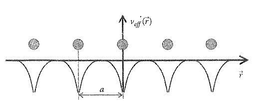
where \(\vec{R}_\ell\) is a lattice vector. It depends on the crystal structure and on the atoms constituting the solid and is called the crystal potential. Schematically, it is shown in Fig. 11.1 in one dimension. The origin for \(\vec{r}\) is generally placed at a lattice point so that one can take full advantage of the point group symmetry of the lattice (see Section 11.6).
It is clear that before we attempt solving the KS equation, we must know \(v_{\text{eff}}(\vec{r})\). Recall that \(v_{\text{eff}}(\vec{r})\) not only includes the electron–ion potential, but also has Hartree and exchange correlation term, that is
\[ \begin{aligned} v_{\text{eff}}(\vec{r}) &= v(\vec{r}) + v_H(\vec{r}) + v_{xc}(\vec{r}) \\ &= -\sum_\ell \frac{1}{4\pi\varepsilon_0}\frac{Ze^2}{|\vec{r} - \vec{R}_\ell|} + \int\frac{1}{4\pi\varepsilon_0}\frac{e^2 n(\vec{r}')}{|\vec{r} - \vec{r}'|}d^3r' + v_{xc}(\vec{r}) \end{aligned} \tag{11.3}\]
where
\[ n(\vec{r}) = \sum_{i,\,\text{occupied}}|\psi_i(\vec{r})|^2 \tag{11.4}\]
For constructing \(v_{\text{eff}}(\vec{r})\), we need \(n(\vec{r})\), which in turn needs the solutions of the KS Eq. 11.1, which we have not solved yet. This problem is generally solved using the following steps:
Start with some guess for \(v_{\text{eff}}(\vec{r})\) and then solve the KS Eq. 11.1.
Once \(\psi_i(\vec{r})\) are known, then obtain \(n(\vec{r})\) using Eq. 11.4 and \(v_{\text{eff}}(\vec{r})\) using Eq. 11.3.
Using the new potential, solve Eq. 11.1 again. One repeats the procedure until convergence is achieved, that is, output potential is the same as the input potential within some tolerance.
In our subsequent discussion, we shall assume that \(v_{\text{eff}}(\vec{r})\) is a given function and focus on how to solve the KS equation with this given potential.
11.3 Bloch’s Theorem
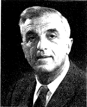
The solution of the KS equation for periodic potential is greatly facilitated by Bloch’s theorem, which was given by Felix Bloch (Fig. 11.2) in 1928 (Bloch 1928). The theorem imposes a condition on the wave function of an electron moving in a periodic potential and is a consequence of the translational symmetry. The theorem can be stated as follows:
For any wave function that satisfies the Schrödinger equation (KS equation) for periodic potential \(v_{\text{eff}}(\vec{r})\) such that \(v_{\text{eff}}(\vec{r} + \vec{R}_\ell) = v_{\text{eff}}(\vec{r})\), there exists a vector \(\vec{k}\) such that translation by a lattice vector \(\vec{R}_\ell\) is equivalent to multiplying by the phase factor \(\exp(i\vec{k}\cdot\vec{R}_\ell)\), that is
\[ \psi_{\vec{k}}(\vec{r} + \vec{R}_\ell) = \exp(i\vec{k}\cdot\vec{R}_\ell)\,\psi_{\vec{k}}(\vec{r}) \tag{11.5}\]
Alternatively, the theorem can also be stated as follows: The wave function should have a form
\[ \psi_{\vec{k}}(\vec{r}) = e^{i\vec{k}\cdot\vec{r}}\,u_{\vec{k}}(\vec{r}) \tag{11.6}\]
where \(u_{\vec{k}}\) is a periodic function, that is
\[ u_{\vec{k}}(\vec{r} + \vec{R}_\ell) = u_{\vec{k}}(\vec{r}) \tag{11.7}\]
To prove the theorem, let us define a translational operator, \(T_\ell\), which when operated on a function \(f(\vec{r})\) translates \(\vec{r}\) by \(\vec{R}_\ell\)
\[ T_\ell f(\vec{r}) = f(\vec{r} + \vec{R}_\ell) \tag{11.8}\]
It can be easily seen that \(T_\ell\) commutes with Hamiltonian \(H(\vec{r})\).
\[ H(\vec{r}) = \left[\frac{-\hbar^2}{2m_e}\nabla^2 + v_{\text{eff}}(\vec{r})\right] \]
that is
\[ \begin{aligned} T_\ell H(\vec{r})\psi(\vec{r}) &= H(\vec{r} + \vec{R}_\ell)\,T_\ell\psi(\vec{r}) \\ &= HT_\ell\psi(\vec{r}) \end{aligned} \]
because \(H(\vec{r})\) has translational symmetry. Thus
\[ T_\ell H = HT_\ell \tag{11.9}\]
This implies that eigenfunctions of \(H\) can be chosen such that those are also eigenfunctions of \(T_\ell\). Therefore, if \(\psi\) is a common eigenfunction
\[ H\psi = \varepsilon\psi \tag{11.10}\]
and
\[ T_\ell\psi = C(\vec{R}_\ell)\psi \tag{11.11}\]
where \(\varepsilon\) and \(C(\vec{R}_\ell)\) are eigenvalues of \(H\) and \(T_\ell\), respectively. Also
\[ \begin{aligned} T_\ell T_{\ell'}\psi(\vec{r}) &= \psi(\vec{r} + \vec{R}_\ell + \vec{R}_{\ell'}) \\ &= T_{\ell+\ell'}\psi(\vec{r}) = T_{\ell'}T_\ell\psi(\vec{r}) \end{aligned} \tag{11.12}\]
Using Eq. 11.11 and Eq. 11.12, we can write
\[ C(\vec{R}_\ell)\,C(\vec{R}_{\ell'}) = C(\vec{R}_\ell + \vec{R}_{\ell'}) \tag{11.13}\]
Let \(\vec{a}_1, \vec{a}_2, \vec{a}_3\) be the primitive vectors of the direct lattice. Let us choose
\[ \vec{R}_\ell = \vec{R}_{\ell'} = \vec{a}_1 \]
Using Eq. 11.13, we can write
\[ C(\vec{a}_1)C(\vec{a}_1) = C(2\vec{a}_1) = C^2(\vec{a}_1) \]
or
\[ C^n(\vec{a}_1) = C(n\vec{a}_1) \tag{11.14}\]
where \(n\) is a positive integer. The form of Eq. 11.14 suggests that
\[ C(\vec{a}_1) = e^{2\pi i x_1} \tag{11.15}\]
where \(x_1\) is a real number. This is because the modulus of \(C(\vec{a}_1)\) must be unity, otherwise Eq. 11.14 will imply an unbounded function. Let us now use the periodic boundary condition
\[ \psi(\vec{r} + N_1\vec{a}_1) = \psi(\vec{r}) \]
where \(N_1, N_2, N_3\) are the number of atoms in the solid along the three basis vectors of the direct lattice such that the total number of atoms in the solid \(N = N_1 N_2 N_3\). The above equation can be written as
\[ T_{N_1\vec{a}_1}\psi(\vec{r}) = \psi(\vec{r}) \tag{11.16}\]
or
\[ C(N_1\vec{a}_1) = 1 \]
This implies from Eq. 11.15
\[ e^{2\pi N_1 i x_1} = 1 = e^{2\pi i m_1} \]
or
\[ x_1 = \frac{m_1}{N_1} \tag{11.17}\]
where \(m_1\) is an integer.
In general
\[ x_i = \frac{m_i}{N_i} \quad (i = 1,2,3) \tag{11.18}\]
Now, \(\vec{R}_\ell\) can be written as
\[ \vec{R}_\ell = \ell_1\vec{a}_1 + \ell_2\vec{a}_2 + \ell_3\vec{a}_3 \tag{11.19}\]
where \(\ell_1, \ell_2, \ell_3\) are integers. Using Eq. 11.15, we can write
\[ C(\vec{R}_\ell) = \exp\!\left[2\pi i\,(\ell_1 x_1 + \ell_2 x_2 + \ell_3 x_3)\right] \tag{11.20}\]
Let us introduce reciprocal lattice vectors \(\vec{b}_1, \vec{b}_2, \vec{b}_3\)
\[ \vec{b}_1 = 2\pi\,\frac{\vec{a}_2\times\vec{a}_3}{\vec{a}_1\cdot(\vec{a}_2\times\vec{a}_3)} \quad \text{etc.} \tag{11.21}\]
which have the property
\[ \vec{b}_i\cdot\vec{a}_j = 2\pi\delta_{ij} \tag{11.22}\]
Let us now define a vector in reciprocal space
\[ \vec{k} = x_1\vec{b}_1 + x_2\vec{b}_2 + x_3\vec{b}_3 \tag{11.23}\]
We see that
\[ \vec{k}\cdot\vec{R}_\ell = 2\pi(\ell_1 x_1 + \ell_2 x_2 + \ell_3 x_3) \tag{11.24}\]
Therefore, Eq. 11.20 can be expressed as
\[ C(\vec{R}_\ell) = e^{i\vec{k}\cdot\vec{R}_\ell} \]
or
\[ T_\ell\psi(\vec{r}) = \psi(\vec{r} + \vec{R}_\ell) = e^{i\vec{k}\cdot\vec{R}_\ell}\psi(\vec{r}) \tag{11.25}\]
This proves Bloch’s theorem.
Here, a few remarks are in order.
The vector \(\vec{k}\) defined in Eq. 11.23, also called a wave vector, is a good quantum number for a periodic system. Thus, the wave functions and energy eigenvalues of an electron in a periodic solid can be labeled by \(\vec{k}\) and written as \(\psi_{\vec{k}}\) and \(\varepsilon_{\vec{k}}\).
As is clear from Eq. 11.5 or Eq. 11.6, if \(\vec{k}\) satisfies Bloch’s theorem, \(\vec{k} + \vec{G}\) also satisfies Bloch’s theorem, where \(\vec{G}\) is a reciprocal lattice vector. Therefore, all possible values of \(\vec{k}\) can be confined to the unit cell of the reciprocal lattice (the first BZ, see Section 11.4 below).
The vector \(\vec{k}\) defined by Bloch’s theorem should not be confused with the vector \(\vec{k}\) occurring in the free electron theory although they play a similar role. The free electron wave vector is given by \(\vec{k} = \vec{p}/\hbar\), where \(\vec{p}\) is the momentum of the electron, while the Bloch wave vector \(\vec{k}\) has no such relationship with the momentum. However, in many processes such as transport and optical absorption, \(\hbar\vec{k}\) behaves as momentum and is called the crystal momentum.
For each \(\vec{k}\), there are several energy eigenvalues that are labeled as \(\varepsilon_{n\vec{k}}\), where \(n\) is called the band index. A detailed plot of \(\varepsilon_{n\vec{k}}\) versus \(\vec{k}\) is referred to as the band structure of the solid.
11.4 Brillouin Zone (BZ)
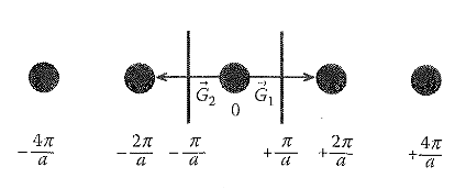
We saw in Section 11.3 that all values of \(\vec{k}\) can be chosen to lie in the primitive unit cell of the reciprocal lattice. Since the primitive unit cell is not unique, it is chosen to be the Wigner–Seitz cell of the reciprocal lattice, which is called the first BZ and is unique. As the name suggests, higher zones can also be constructed, but we shall limit ourselves to the first Brillouin zone or simply Brillouin zone. It is constructed in the following way: (i) Choose a reciprocal lattice point as origin. (ii) Connect all the remaining points to the origin, drawing all the reciprocal lattice vectors and label them as \(\vec{G}_1, \vec{G}_2, \vec{G}_3\), and so on. For the first BZ, there is no need to go beyond the third next neighbor. (iii) Draw perpendicular bisector planes to \(\vec{G}_1, \vec{G}_2, \vec{G}_3\), and so on. (iv) The smallest polyhedron containing the origin is the first BZ. We first demonstrate it by an example of one-dimensional lattice constant \(a\). Its reciprocal lattice is also a one-dimensional lattice with lattice constant of \(2\pi/a\). We see that the first nearest neighbors of 0 are at \(\pm 2\pi/a\) as shown in Fig. 11.3. By drawing the perpendicular bisectors, we find that the first BZ lies between \(\pm\pi/a\).
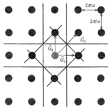
Another example we take is of a square lattice of lattice constant \(a\). It can be shown that the reciprocal lattice of a square lattice is also a square lattice with lattice constant \(2\pi/a\) as shown in Fig. 11.4. Now, choose a point as origin and draw reciprocal lattice vectors \(\vec{G}_1, \vec{G}_2, \vec{G}_3\), and so on. We see that the smallest area contained by the perpendicular bisectors is the shaded square with sides of length \(2\pi/a\). Thus, all \(\vec{k}\) vectors are contained within \((\pm\pi/a,\,\pm\pi/a)\).
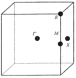
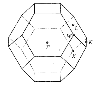
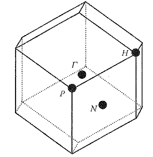
In a similar way, one can construct BZ in three dimensions. The BZs for simple cubic, fcc, and bcc lattices are shown in Fig. 11.5, Fig. 11.6, and Fig. 11.7 respectively. Various symmetry points have been labeled by standard symbols. For example, \(\Gamma\) denotes (0,0,0), \(M\) is (110), \(X\) is (100), and \(R\) is (111) for the BZ of a cubic lattice. The coordinates are with respect to a Cartesian frame fixed at \(\Gamma\) and are in units of \(2\pi/a\). The energy bands are generally plotted along the lines joining these symmetry points.
The planes at the surface of the BZ have some special significance. A wave vector \(\vec{k}\) whose tip is lying on these planes satisfies the equation
\[ \vec{k}\cdot\vec{G} = \frac{1}{2}G \]
where \(\vec{G}\) is a reciprocal lattice vector (see Kittel (1986) or Ashcroft and Mermin (1976)). This is nothing but Bragg or Laue’s condition for maxima in x-ray diffraction. Thus, the bounding planes of the BZ are the Bragg planes. We shall see in the next chapter that an electron wave with wave vector corresponding to a Bragg plane will get strongly reflected and will strongly interfere with the incoming wave. This gives rise to an energy band gap at the wave vectors corresponding to these planes.
11.5 Spin–Orbit Interaction
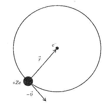
The spin and orbital angular momentum of an electron can couple together and give rise to an additional term in the Hamiltonian, known as the spin–orbit interaction. Although this is a relatively weak interaction, it can have pronounced effects in materials where one of the constituent atoms is a heavy element. This is basically a relativistic effect and can be derived from the Dirac equation. However, here, we shall derive it by using a simple semiclassical argument that makes it clear why there should be coupling between spin of the electron and its orbital angular momentum. Let us consider a hydrogen-like atom with an electron (charge \(-e\)) moving in a circular orbit of radius \(r\) around its nucleus with charge \(+Ze\), as shown in Fig. 11.8. Let us assume that its spin and orbital angular momenta are \(\vec{S}\) and \(\vec{L}\).
Because of spin angular momentum \(\vec{S}\), the electron has a magnetic moment \(\vec{\mu}\)
\[ \vec{\mu} = -\frac{e\vec{S}}{m_e} \tag{11.26}\]
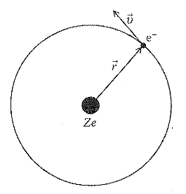
where \(m_e\) is its mass (Eisberg and Resnick 1974). To see the coupling between \(\vec{S}\) and \(\vec{L}\), let us go to the rest frame of the electron. In this frame, the electron is at rest and the nucleus is moving with velocity \(-\vec{v}\) as shown in Fig. 11.9. Since the nucleus with charge \(+Ze\) is moving, it gives rise to a current in this frame. A current element is given by
\[ id\vec{\ell} = \frac{dq}{dt}\,d\vec{\ell} = dq\,\frac{d\vec{\ell}}{dt} = -Ze\vec{v} \tag{11.27}\]
This current element gives rise to a magnetic field \(\vec{B}\) at the location of the electron, given by the Biot–Savart law as
\[ \vec{B} = \frac{\mu_0}{4\pi}\frac{id\vec{\ell}\times\vec{r}}{r^3} = -\frac{\mu_0}{4\pi}\frac{Ze\vec{v}\times\vec{r}}{r^3} \tag{11.28}\]
Let us write this in terms of the electric field created by the nucleus at \(\vec{r}\)
\[ \vec{E} = \frac{Ze\vec{r}}{4\pi\varepsilon_0 r^3} = \frac{1}{er}\frac{dV(r)}{dr}\vec{r} \tag{11.29}\]
where \(V(r)\) is the potential energy of the electron at \(\vec{r}\)
\[ V(r) = -\frac{Ze^2}{4\pi\varepsilon_0 r} \]
This gives
\[ \vec{B} = -\varepsilon_0\mu_0\vec{v}\times\vec{E} = -\frac{1}{c^2}\vec{v}\times\vec{E} \tag{11.30}\]
where \(c = 1/\sqrt{\varepsilon_0\mu_0}\) is the speed of light in vacuum. The magnetic field Eq. 11.30 interacts with the magnetic moment of the electron with interaction energy
\[ \begin{aligned} \Delta E &= -\vec{\mu}\cdot\vec{B} \\ &= -\frac{e}{m_e c^2}\vec{S}\cdot(\vec{v}\times\vec{E}) \\ &= -\frac{1}{m_e rc^2}\left(\vec{v}\times\frac{dV}{dr}\vec{r}\right)\cdot\vec{S} \\ &= \frac{1}{m_e^2 c^2}\frac{1}{r}\frac{dV(r)}{dr}(\vec{r}\times m_e\vec{v})\cdot\vec{S} \end{aligned} \tag{11.31}\]
where we have used Eq. 11.29. Now substituting
\[ \vec{L} = \vec{r}\times m_e\vec{v} \]
we get
\[ \Delta E = \frac{1}{m_e^2 c^2 r}\frac{dV}{dr}\,\vec{L}\cdot\vec{S} \tag{11.32}\]
This is the interaction energy in the rest frame of the electron, while we are interested in the frame in which the nucleus is at rest. Because of the relativistic transformation of velocities, the transformation back to the normal frame reduces the interaction energy by a factor of 2 (Eisberg and Resnick 1974). Thus, the spin–orbit interaction can be written as
\[ H_{SO} = \frac{1}{2m_e^2 c^2}\frac{1}{r}\frac{dV(r)}{dr}\,\vec{S}\cdot\vec{L} \tag{11.33}\]
Although this expression has been derived semi-classically, this is in complete agreement with the expression obtained from the Dirac equation. This interaction given by Eq. 11.33 is small compared to \(V(r)\) and can be treated as a small perturbation. Using the hydrogen-like wave functions, it can be shown that the first-order change in energy of an atom goes as \(Z^4\), where \(Z\) is the atomic number (Landau and Lifshitz 1977). This shows that spin–orbit interaction could be quite important for heavy elements.
It turns out that the expression (Eq. 11.33), which was derived for a hydrogen-like atom, is also applicable to solids and molecules. Eq. 11.33 can be rewritten as
\[ \begin{aligned} H_{SO} &= \frac{e}{2m_e^2 c^2}\vec{S}\cdot(\vec{E}\times\vec{p}) \\ &= -\frac{e}{2m_e^2 c^2}\vec{E}\cdot(\vec{S}\times\vec{p}) \end{aligned} \]
where we have used Eq. 11.29. In solids, the spin–orbit interaction can be large if the electric field, \(\vec{E}\), experienced by the electron is large. This can happen if the electron is near a nucleus, a surface, or an interface. In solids, the spin–orbit interaction often splits the degenerate levels at the symmetry points of the BZ. We shall see in later Chapter that the spin–orbit interaction plays an important role in topological insulators.
The full one-electron Hamiltonian can be written as
\[ H = H_0 + \frac{e\hbar}{4m_e^2 c^2}\vec{\sigma}\cdot(\vec{E}\times\vec{p}) \tag{11.34}\]
where we have written that \(\vec{S} = (\hbar/2)\vec{\sigma}\) and \(H_0\) contains the kinetic energy and other potential excluding spin–orbit term. \(\vec{\sigma}\) are Pauli spin matrices given by
\[ \sigma_x = \begin{pmatrix}0 & 1\\1 & 0\end{pmatrix},\quad \sigma_y = \begin{pmatrix}0 & -i\\i & 0\end{pmatrix},\quad \sigma_z = \begin{pmatrix}1 & 0\\0 & -1\end{pmatrix} \tag{11.35}\]
The pure spin states \(\alpha\) and \(\beta\) are
\[ \alpha = \begin{pmatrix}1\\0\end{pmatrix} \quad \text{and} \quad \beta = \begin{pmatrix}0\\1\end{pmatrix} \tag{11.36}\]
The spin–orbit interaction mixes spin states \(\alpha\) and \(\beta\).
Since Hamiltonian Eq. 11.34 is translationally invariant, eigenfunctions of \(H\) can be labeled by \(\vec{k}\), which can be written as
\[ \psi_{\vec{k}\uparrow}(\vec{r}) = \chi_{\vec{k}\uparrow}(\vec{r})\alpha + \gamma_{\vec{k}\uparrow}(\vec{r})\beta \]
and
\[ \psi_{\vec{k}\downarrow}(\vec{r}) = \chi_{\vec{k}\downarrow}(\vec{r})\alpha + \gamma_{\vec{k}\downarrow}(\vec{r})\beta \tag{11.37}\]
where \(\uparrow\) denotes a state with the spin generally up, that is, its projection onto \(\alpha\) is positive. \(\chi_{\vec{k}\uparrow}\) and \(\gamma_{\vec{k}\uparrow}\) are the space part of the wave function.
11.6 Symmetry
Symmetry plays an important role in the energy band theory. It allows one to classify and label the eigenstates and eigenvalues of a Hamiltonian as we have seen in Section 11.3 for translational symmetry. Symmetry can predict degeneracy of levels at symmetry points of the BZ. It can also predict certain transition probabilities and matrix elements between two states to be zero and can produce selection rules. In the electronic structure calculations, the use of symmetry can reduce the numerical effort tremendously.
In addition to the translational symmetry, a crystal can have rotational symmetries about various axes, mirror symmetries about certain planes, and inversion symmetry. These symmetries are called point group symmetries because in all point group operations, a point is kept fixed. All symmetry elements of a crystal form a group called a point group. Only 32 different point groups are possible for crystalline solids. Since the Hamiltonian is invariant under point group operations, the energy level \(\varepsilon_{n\vec{k}}\) has the full point group symmetry in the reciprocal space as we shall see below.
Let \(S\) denote a point group symmetry operation that transforms \(\vec{r}\) to \(\vec{r}'\), that is
\[ \vec{r}' = S\vec{r} \tag{11.38}\]
where \(S\) is a unitary matrix. This is because the operation does not change the magnitude of \(\vec{r}\). The symmetry operation changes function \(f(\vec{r})\) as
\[ Sf(\vec{r}) = f(S\vec{r}) \tag{11.39}\]
Let \(\sigma\) denote up or down spin and \(\psi_{\vec{k}\sigma}(\vec{r})\) and \(\varepsilon_{\vec{k}\sigma}\) an eigenfunction and eigenvalue of the Hamiltonian \(H\), respectively. For simplicity, we have suppressed the band index \(n\). Since \(S\) is a symmetry operation, \(H\) remains invariant under this operation. This implies that \(H\) and \(S\) commute, that is
\[ HS = SH \tag{11.40}\]
Thus
\[ HS\psi_{\vec{k}\sigma}(\vec{r}) = SH\psi_{\vec{k}\sigma}(\vec{r}) \]
or
\[ H[S\psi_{\vec{k}\sigma}(\vec{r})] = \varepsilon_{\vec{k}\sigma}[S\psi_{\vec{k}\sigma}(\vec{r})] \tag{11.41}\]
Eq. 11.41 implies that \(S\psi_{\vec{k}\sigma}(\vec{r})\) and \(\psi_{\vec{k}\sigma}(\vec{r})\) have the same energy \(\varepsilon_{\vec{k}\sigma}\). Bloch’s theorem implies that
\[ \psi_{\vec{k}\sigma}(\vec{r} + \vec{R}) = e^{i\vec{k}\cdot\vec{R}}\psi_{\vec{k}\sigma}(\vec{r}) \]
Thus
\[ \begin{aligned} S\psi_{\vec{k}\sigma}(\vec{r} + \vec{R}) &= \psi_{\vec{k}\sigma}(S(\vec{r}+\vec{R})) = \psi_{\vec{k}\sigma}(S\vec{r} + S\vec{R}) \\ &= e^{i\vec{k}\cdot S\vec{R}}\psi_{\vec{k}\sigma}(S\vec{r}) \end{aligned} \tag{11.42}\]
This is because \(S\vec{R}\) is a lattice vector. Also, we note that if we apply the same symmetry operation to both vectors, \(\vec{k}\) and \(S\vec{R}\), their scalar product remains unchanged (e.g., if we rotate both vectors by the same angle). Thus
\[ \vec{k}\cdot S\vec{R} = S^{-1}\vec{k}\cdot S^{-1}S\vec{R} = S^{-1}\vec{k}\cdot\vec{R} \tag{11.43}\]
Using Eq. 11.43, Eq. 11.42 can be written as
\[ \psi_{\vec{k}\sigma}(S(\vec{r}+\vec{R})) = e^{iS^{-1}\vec{k}\cdot\vec{R}}\psi_{\vec{k}\sigma}(S\vec{r}) \tag{11.44}\]
This implies that \(\psi_{\vec{k}\sigma}(S\vec{r})\) is an eigenfunction of the translational operator with wave vector \(S^{-1}\vec{k}\) and corresponds to the same energy \(\varepsilon_{\vec{k}\sigma}\). Thus, we have
\[ \psi_{\vec{k}\sigma}(S\vec{r}) = \psi_{S^{-1}\vec{k}\sigma}(\vec{r}), \qquad \varepsilon_{S^{-1}\vec{k}\sigma} = \varepsilon_{\vec{k}\sigma} \tag{11.45}\]
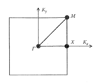
The above discussion implies that many \(\vec{k}\) points in the BZ, which are connected by the point group symmetry operations, have the same energy. Thus, it is useful to define the irreducible Brillouin zone (IBZ), which is much smaller than the BZ, such that all points outside the IBZ are connected with \(\vec{k}\) points in the IBZ by some point group symmetry. For example, the IBZ of a square lattice is shown in Fig. 11.10, which is 1/8th of the full zone. For a cubic system, the IBZ is 1/48th of the full zone. Thus, if one wants to integrate a function that has the cubic point group symmetry, one needs to integrate only over 1/48 of the BZ. Thus, the use of symmetry can reduce numerical effort by an enormous amount.
If we add translations to the point group operations, the resulting symmetry elements form a group called a space group. There are only 230 different space groups possible. We shall not go into the details of the group theory but refer to some excellent books such as by Heine (1960), Tinkham (1964), and Falicov (1966). These space groups have been assigned unique symbols and a number identifying them (see, e.g., Hahn 2002). All electronic structure studies use space group symmetries to simplify calculations; therefore, information about the space group is an input to these calculations.
11.7 Inversion Symmetry, Time Reversal, and Kramers’ Theorem
Inversion symmetry means that if we change \(\vec{r}\) to \(-\vec{r}\), the system remains invariant. Let us define an operator \(I\) that performs the inversion operation. If the Hamiltonian is invariant under inversion, \(I\) and \(H\) commute, that is
\[ HI = IH \tag{11.46}\]
Thus, if \(\psi_{\vec{k}\sigma}\) is an eigenfunction of \(H\) with energy \(\varepsilon_{\vec{k}\sigma}\) and spin \(\sigma\), then
\[ \begin{aligned} HI\psi_{\vec{k}\sigma} &= IH\psi_{\vec{k}\sigma} \\ &= I\varepsilon_{\vec{k}\sigma}\psi_{\vec{k}\sigma} \end{aligned} \]
or
\[ H(I\psi_{\vec{k}\sigma}) = \varepsilon_{\vec{k}\sigma}(I\psi_{\vec{k}\sigma}) \tag{11.47}\]
Thus, \(I\psi_{\vec{k}\sigma}\) is also an eigenfunction of \(H\) with energy \(\varepsilon_{\vec{k}\sigma}\). To identify the wave vector of \(I\psi_{\vec{k}\sigma}\), we use Bloch’s theorem, which gives
\[ I\psi_{\vec{k}\sigma}(\vec{r}+\vec{R}) = e^{-i\vec{k}\cdot\vec{R}}\psi_{\vec{k}\sigma}(-\vec{r}) = e^{-i\vec{k}\cdot\vec{R}}I\psi_{\vec{k}\sigma}(\vec{r}) \]
This implies that \(I\psi_{\vec{k}\sigma}\) corresponds to wave vector \(-\vec{k}\) and energy \(\varepsilon_{-\vec{k}\sigma}\). But according to Eq. 11.47, this is equal to \(\varepsilon_{\vec{k}\sigma}\). Thus, the inversion symmetry implies that
\[ \varepsilon_{-\vec{k}\sigma} = \varepsilon_{\vec{k}\sigma} \tag{11.48}\]
This is an important result of inversion symmetry, which means that we do not have to calculate bands for negative values of wave vectors, if the system has inversion symmetry.
Now, we discuss the time-reversal symmetry, which means that the Hamiltonian remains invariant as time \(t\) is replaced by \(-t\). We see that the Hamiltonian \(H\) (Eq. 11.34) has the time-reversal symmetry. This is because on time reversal the direction of spin \(\vec{S}\) as well as the momentum \(\vec{p}\) reverses. Let \(T\) denote the time-reversal operator. Kramers’ theorem states that if \(\psi_{\vec{k}\sigma}\) is a one-electron eigenstate of \(H\), then \(T\psi_{\vec{k}\sigma}\) is also an eigenstate with the same energy in the absence of the external magnetic field. Also, \(T\psi_{\vec{k}\sigma}\) is orthogonal to \(\psi_{\vec{k}\sigma}\).
Since \(H\) is invariant under time-reversal, \(T\) commutes with \(H\), that is
\[ HT = TH \tag{11.49}\]
This implies that if \(\psi_{\vec{k}\sigma}\) is an eigenfunction of \(H\) with energy \(\varepsilon_{\vec{k}\sigma}\), then
\[ \begin{aligned} HT\psi_{\vec{k}\sigma} &= TH\psi_{\vec{k}\sigma} \\ &= T\varepsilon_{\vec{k}\sigma}\psi_{\vec{k}\sigma} \end{aligned} \]
or
\[ H(T\psi_{\vec{k}\sigma}) = \varepsilon_{\vec{k}\sigma}(T\psi_{\vec{k}\sigma}) \]
that is, \(T\psi_{\vec{k}\sigma}\) is also an eigenfunction of \(H\) with energy \(\varepsilon_{\vec{k}\sigma}\).
\(T\) transforms \(\psi_{\vec{k}\sigma}\) into \(\psi_{-\vec{k},-\sigma}\) because by reversing \(t\) the momentum and spin are reversed. Since these two eigenvectors belong to different eigenvalues of the translational operator, they are orthogonal to each other. This proves the theorem.
Thus
\[ T\psi_{\vec{k}\uparrow} = \psi_{-\vec{k}\downarrow} \]
and
\[ T\psi_{\vec{k}\downarrow} = \psi_{-\vec{k}\uparrow} \tag{11.50}\]
This further implies from Kramers’ theorem that
\[ \varepsilon_{\vec{k}\uparrow} = \varepsilon_{-\vec{k}\downarrow} \]
and
\[ \varepsilon_{\vec{k}\downarrow} = \varepsilon_{-\vec{k}\uparrow} \tag{11.51}\]
that is, there is a twofold degeneracy in the bands. If there is no spin–orbit coupling, then in the absence of a magnetic field, \(\varepsilon_{\vec{k}\uparrow} = \varepsilon_{\vec{k}\downarrow}\) and all the energies in Eq. 11.51 are the same. This implies that \(\varepsilon_{\vec{k}\sigma} = \varepsilon_{-\vec{k}\sigma}\), which is an important consequence of the time-reversal symmetry and holds even if there is no inversion symmetry.
In the presence of the external magnetic field \(\vec{B}\), the Hamiltonian will have a term like \(\vec{S}\cdot\vec{B}\). Since \(T\) will reverse \(\vec{S}\), it will no longer commute with \(H\), or in other words the magnetic field breaks the time-reversal symmetry. Therefore, Kramers’ theorem does not hold in the presence of the magnetic field.
11.8 Band Structure and Fermi Surface
For each \(\vec{k}\), there are many eigenvalues of \(H\) that are labeled as \(\varepsilon_{n\vec{k}}\), where \(n\) is a band index. A plot of \(\varepsilon_{n\vec{k}}\) versus \(\vec{k}\) is called band structure. There are many methods for calculating band structure, which we will discuss in the next few chapters. Here, we shall discuss some main features of band structure.
One very important result of band theory is that in the band structure of a crystalline solid, we have allowed ranges of energy, called energy bands. The forbidden ranges of energy are called energy band gaps. In the next chapter, we shall discuss in detail the origin of energy band gaps. When discussing the nearly free electron model, we shall see that the band gaps arise due to the quantum interference of electron waves moving in a periodic lattice, very similar to the interference of electromagnetic waves. Another way to understand it is to look at this from the perspective of the tight-binding model. We bring the atoms from infinity to a very small distance on a periodic lattice and see how the atomic levels evolve into bands. We shall discuss it in detail in Chapter Section 12.1.
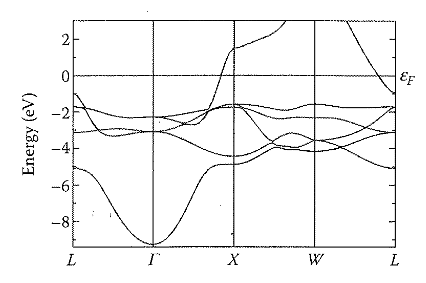
As an example, we show the band structure of copper in Fig. 11.11, along various symmetry lines in the BZ. \(\Gamma\), \(X\), \(W\), and so on are various symmetry points in the BZ shown in Fig. 11.6 and the band structure is plotted along the lines joining these points. The band structure of copper was obtained by using the Vienna ab initio simulation package (VASP) code (Kresse and Furthmüller 1996a,b). The lattice constant was taken to be 3.6309 Å and the energy cutoff, 400 eV with \(18\times18\times18\) Monkhorst–Pack \(k\)-mesh (Monkhorst and Pack 1976). In the figure, the highest filled level, called Fermi energy, is denoted by \(\varepsilon_F\) and taken as the zero of energy. The \(d\) bands lie in the narrow energy range of approximately \(-2\) to \(-4\) eV. We see that the \(d\) bands are quite flat. The \(s\)–\(p\) type bands have parabolic shape and lie in the energy range of \(-10\) to \(-5\) eV and 0 to 2 eV. In the region of the \(d\) bands, there is a mixing of \(s\) states with the \(d\) states, and this is known as \(s\)–\(d\) hybridization. Owing to the \(s\)–\(d\) hybridization, the lowest band starting from \(\Gamma\), which has parabolic shape up to about \(-5\) eV, changes to a flatter band up to \(X\) or \(L\). The band structure can be measured by ARPES. The experimental band structure of Cu obtained by ARPES has been found in excellent agreement with theoretical calculations (Courths and Hufner 1984).
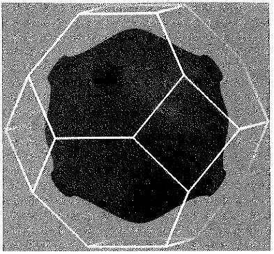
The one-electron levels \(\varepsilon_{n\vec{k}}\) are filled in accordance with the Pauli exclusion principle. As we had defined earlier, the Fermi energy, \(\varepsilon_F\), is the highest filled level in the band structure at absolute zero temperature. The constant energy surface in \(\vec{k}\) space corresponding to \(\varepsilon_F\) is known as the Fermi surface. The Fermi surface of copper is shown in Fig. 11.12. As we can see, it is very different from a sphere. This is because there is \(s\)–\(d\) hybridization and the band intersecting the Fermi energy is not purely \(s\)–\(p\) type but also has \(d\) character. It has a neck-like structure around point \(L\) and is not a closed surface. The Fermi surface, in general, can have a very complex structure. For example, Nb, Mo, and Ni have a very complicated Fermi surface (see, e.g., Rajput et al. 1996, Prasad et al. 1977). The Fermi surface can be measured by the de Haas–van Alphen (dHvA) method. This is a very accurate method for measuring Fermi surface, but requires very pure single crystal samples and very low temperatures. Another method is the two-dimensional angular correlation of positron annihilation radiation (2D-ACAR). This method does not require pure samples and low temperatures but is not as accurate as the dHvA. The Fermi surfaces of disordered alloys have been measured by this method.
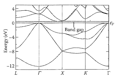
We see that in copper, bands are partially filled. Such materials with partially filled bands are metals, as a small application of electric field can produce a current. Band theory can predict whether a material is a metal or insulator at absolute zero. If the bands are partially filled, as is the case for copper, it is a metal because the application of an electric field would produce a current. It can be shown that a filled band cannot contribute to the current (see Exercise 11.8). Thus, if a material has completely filled bands, as is the case in carbon, it would be an insulator, at absolute zero. However, if the band gap between the highest filled band and lowest unoccupied band is \(<2\) eV, the electrons can get thermally excited across the band gap at room temperature. Now, both bands are partially filled and as a result the material will conduct. Such a material is called a semiconductor. In Fig. 11.13, we show the band structure of silicon, which is a typical example of a semiconductor. The band structure was calculated by using the VASP code (Kresse and Furthmüller 1996a,b). The lattice constant was taken to be 5.43 Å and the energy cut off, 250 eV with \(20\times20\times20\) Monkhorst–Pack \(k\)-mesh (Monkhorst and Pack 1976). We see that above the fully filled band there is a band gap shown by the shaded region. We see that the minimum band gap occurs between energy eigenvalues at two different \(\vec{k}\)-points. This is called indirect band gap and the corresponding material is called indirect band gap semiconductor as opposed to direct band gap semiconductor in which the minimum band gap occurs at the same \(\vec{k}\)-point.
The ability of band theory to predict the metallic or insulating behavior of a material has been one of its great achievements. However, it may fail if the material is a strongly correlated material such as NiO, CoO, MnO, or high-\(T_c\) cuprates.
11.9 Density of States, Local Density of States, and Projected Density of States
One very useful quantity that we will frequently encounter in electronic structure studies is the density of states (DOS). The DOS is defined as the number of states per unit energy range per unit cell
\[ \rho(\varepsilon) = \frac{dN}{d\varepsilon} \tag{11.52}\]
where \(dN\) is the number of states per unit cell in the energy range \(\varepsilon\) and \(\varepsilon + d\varepsilon\). An alternative definition is
\[ \rho(\varepsilon) = \frac{1}{N_{cell}}\sum_{\vec{k},n}\delta(\varepsilon - \varepsilon_{n\vec{k}}) \tag{11.53}\]
where \(N_{cell}\) is the number of unit cells in the solid. Note that in case of the free electron model, the DOS was defined such that its unit was number of states per unit energy per unit volume. However, in general, it is defined using Eq. 11.53 such that its unit is number of states per unit energy per unit cell. The DOS is an important quantity that appears in various calculations such as calculation of specific heat, transport properties, and so on. It shows singularities known as van Hove singularities (see Exercise 11.10).
Another important quantity of interest is local density of states (LDOS). Suppose all the atoms in the solid are not equivalent and we would like to know the contribution of one particular atom to the total DOS. For this purpose, let us assume that we know an orthonormal set of atomic wave functions \(|\phi_\ell\rangle\) centered on site \(\ell\), so that we can expand the Bloch wave functions \(|\psi_{n\vec{k}}\rangle\) as:
\[ |\psi_{n\vec{k}}\rangle = \sum_\ell\langle\phi_\ell|\psi_{n\vec{k}}\rangle\,|\phi_\ell\rangle \tag{11.54}\]
where
\[ \langle\phi_\ell|\psi_{n\vec{k}}\rangle = \int_\ell\phi_\ell^*(\vec{r})\,\psi_{n\vec{k}}(\vec{r})\,d^3r \tag{11.55}\]
where the integration is over the volume around atom \(\ell\). This implies that the probability of finding an electron with wave vector \(\vec{k}\) and energy \(\varepsilon_{n\vec{k}}\) in state \(|\phi_\ell\rangle\) is \(|\langle\phi_\ell|\psi_{n\vec{k}}\rangle|^2\). Thus, contribution of the state \(|\phi_\ell\rangle\) to the DOS coming from \(\psi_{n\vec{k}}\) has to be weighted by \(|\langle\phi_\ell|\psi_{n\vec{k}}\rangle|^2\). Then, the LDOS, which is the contribution of site \(\ell\) to the total DOS, is defined as
\[ \rho_\ell(\varepsilon) = \frac{1}{N_{cell}}\sum_{\vec{k},n}\left|\langle\phi_\ell|\psi_{n\vec{k}}\rangle\right|^2\delta(\varepsilon - \varepsilon_{n\vec{k}}) \tag{11.56}\]
The unit of LDOS is the number of states per unit energy per atom. Note that the total DOS is the sum of LDOS coming from all atoms
\[ \begin{aligned} \rho(\varepsilon) &= \sum_\ell\rho_\ell(\varepsilon) = \frac{1}{N_{cell}}\sum_{\vec{k},n,l}\left|\langle\phi_\ell|\psi_{n\vec{k}}\rangle\right|^2\delta(\varepsilon - \varepsilon_{n\vec{k}}) \\ &= \frac{1}{N_{cell}}\sum_{n\vec{k}}\delta(\varepsilon - \varepsilon_{n\vec{k}}) \end{aligned} \tag{11.57}\]
This is because
\[ \sum_\ell\left|\langle\phi_\ell|\psi_{n\vec{k}}\rangle\right|^2 = 1 \tag{11.58}\]
The above idea can be generalized to define projected density of states (PDOS), which is the angular momentum decomposition of the LDOS. We expand the Bloch wave function \(|\psi_{n\vec{k}}\rangle\), in terms of orthonormal set \(|\phi_{\ell L}\rangle\), where \(L\) is the composite angular momentum index for \((l, m)\). Thus
\[ |\psi_{n\vec{k}}\rangle = \sum_{\ell,L}\langle\phi_{\ell L}|\psi_{n\vec{k}}\rangle\,|\phi_{\ell L}\rangle \tag{11.59}\]
Thus, we can define PDOS as
\[ \rho_{\ell L}(\varepsilon) = \frac{1}{N_{cell}}\sum_{\vec{k},n}\left|\langle\phi_{\ell L}|\psi_{n\vec{k}}\rangle\right|^2\delta(\varepsilon - \varepsilon_{n\vec{k}}) \tag{11.60}\]
PDOS is an important quantity to find the angular momentum character of LDOS as we shall see below. Note that the definition of PDOS and LDOS has a matrix element such as Eq. 11.55, whose evaluation involves integral over volume around atom \(\ell\). The integral is generally evaluated over a spherical volume of radius equal to the Wigner–Seitz radius. Since one cannot unambiguously assign a volume to an atom in a solid containing different kinds of atoms, this leads to some uncertainty. Nevertheless, LDOS and PDOS are very useful quantities as we shall see later.
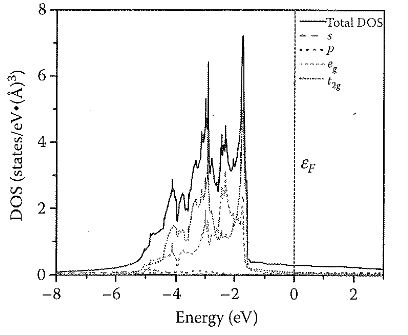
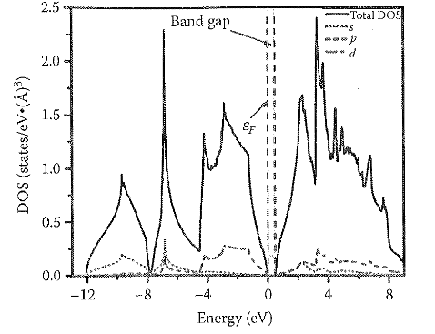
As examples, we show the DOS and PDOS of copper and silicon in Fig. 11.14 and Fig. 11.15, respectively. For copper, we see a large density of states in the energy range \(-3\) to \(-1\) eV, which is mainly contributed by \(d\) states (\(e_g\) and \(t_{2g}\)) as can be seen from \(d\) PDOS. However, at the Fermi energy, the contribution of \(d\) states to DOS gets reduced. In silicon, we see that in the band gap, the DOS is zero. In other words, by looking at the range of zero DOS we can find the band gap. Here, the band gap is about 0.5 eV, which is much smaller than the experimental gap of about 1.1 eV. This is due to the use of LDA, which leads to a much smaller band gap as mentioned in previous chapters . This can be corrected by using a better functional or GW method.
11.10 Charge Density
The charge density at location \(\vec{r}\) is defined as
\[ \rho(\vec{r}) = -e\sum_{n,\vec{k},\,\text{occupied}}|\psi_{n\vec{k}}(\vec{r})|^2 = -en(\vec{r}) \tag{11.61}\]
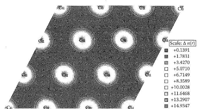
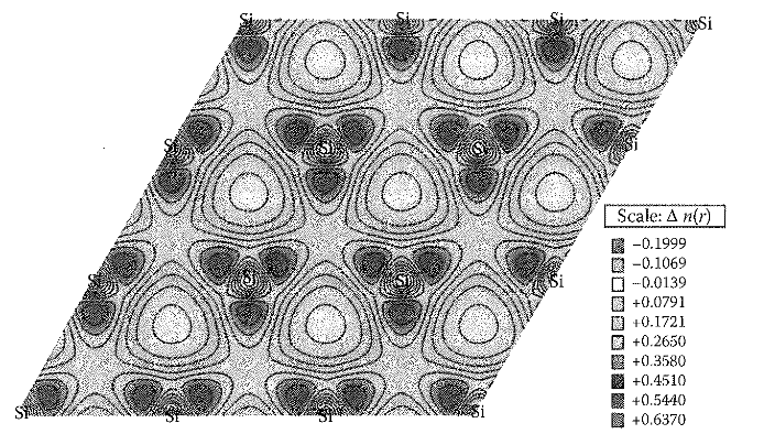
where \(e\) is the electronic charge and \(n(\vec{r})\) the electron density. Here, the sum is over all the occupied states. The charge density can be measured by using x-ray diffraction. As we have seen, the electron density \(n(\vec{r})\) plays a central role in the DFT. The distribution of electronic charge in a solid can give important information about the type of bonding. For example, in metals, the charge density is quite isotropic around an atom, while in covalent solids, it is highly directional. In Fig. 11.16, we show the charge density for copper in (100) plane and we can see that the charge density in copper around an atom is quite isotropic in contrast to the charge density in silicon, which is highly directional as seen in Fig. 11.17.
11.11 Brillouin Zone Integration
For many calculations such as the calculation of the total energy, charge density, and the DOS, one has to sum over \(\vec{k}\), which can be converted to a BZ integration such as
\[ \sum_{\vec{k}}f(\vec{k}) = \frac{\Omega}{8\pi^3}\int_{BZ}f(\vec{k})\,d^3k \tag{11.62}\]
where \(\Omega\) is the volume of the solid. This integral for a real material has to be evaluated numerically. The numerical effort can be reduced considerably by exploiting the point group symmetry of the system. If the integrand \(f(\vec{k})\) has point group symmetry, the integral has to be done only over the irreducible part of the Brillouin zone (IBZ), which has much smaller volume compared to the full BZ. For numerical integration, the BZ integral is evaluated by summing over discrete set of \(\vec{k}\) points. For efficient calculation of integral over BZ, several methods have been developed. The choice of method depends on whether the system is an insulator or a metal. For insulators, all occupied bands are full; therefore, the function \(f(\vec{k})\) is generally a smooth function of \(\vec{k}\). Thus, the evaluation of such BZ integrals for insulators requires a smaller number of \(\vec{k}\) points than the number required for metals. For a metal, function \(f(\vec{k})\), which involves the sum over the occupied states, will have discontinuity at the Fermi surface. This requires careful handling, and in general, one will require a larger number of \(\vec{k}\) points for an accurate evaluation. Various methods suggested for BZ integration are special \(\vec{k}\)-point methods (Baldereschi 1973, Chadi and Cohen 1973, Monkhorst and Pack 1976), the Methfessel and Paxton method (Methfessel and Paxton 1989), the tetrahedron method (Jepsen and Andersen 1971, Blochl and Andersen 1994), the special directions method (Bansil 1975, Prasad and Bansil 1980), and so on. We shall not go into the details of these methods and refer the reader to the original papers.
11.12 Exercises
Show that all possible values of \(\vec{k}\) can be confined to the first BZ.
Show that the number of allowed wave vectors \(\vec{k}\) in the BZ is equal to the number of sites in the solid.
Using the spin–orbit interaction as perturbation, show that the first-order change in energy of an atom goes as \(Z^4\), where \(Z\) is the atomic number. You may use hydrogen-like wave functions in your calculation.
Consider a rectangular lattice with \(a = 4\) Å and \(b = 8\) Å. Draw the Brillouin zone and clearly show the IBZ.
Draw the BZs of simple cubic, fcc, and bcc lattices using the cube edge \(a = 4\) Å. In the figure, mark the coordinates of symmetry points using standard symbols.
Show that the periodic part of the Bloch wave function \(u_{\vec{k}}(\vec{r})\) satisfies the equation
\[ \left( \frac{\hbar^2}{2m_e} \left( \frac{\vec{\nabla}}{i}+\vec{k} \right)^2 +v(\vec{r}) \right) u_{\vec{k}}(\vec{r}) = \varepsilon_{\vec{k}}u_{\vec{k}}(\vec{r}) \]
Using the result of Exercise 11.6, show that the mean velocity of an electron in level \(\varepsilon_{n\vec{k}}\) is given by
\[ \vec{v}_n(\vec{k}) = \frac{1}{\hbar} \vec{\nabla}_{\vec{k}} (\varepsilon_{n\vec{k}}) \]
Using the result of Exercise 11.7, show that a filled band does not contribute to the current density.
Show that the density of states can be written as
\[ \rho(\varepsilon) = \int_s \frac{ds}{4\pi^3} \frac{1} {\left| \vec{\nabla}_{\vec{k}} (\varepsilon_{\vec{k}}) \right|} \]
where the integral is over a constant energy surface \(\varepsilon=\varepsilon_{\vec{k}}\).
Exercise 11.9 implies that \(\rho(\varepsilon)\) will have singularities. However, in 3D, these singularities are integrable and give finite results for \(\rho(\varepsilon)\) but the slope has divergences. These singularities are known as van Hove singularities.
Consider the following case when
\[ \varepsilon_{\vec{k}} = \varepsilon_o + \alpha_1 (k_x^2+k_y^2) + \alpha_2 k_z^2 \]
Using the result given in Exercise 11.9, show that \(\rho(\varepsilon)\) is finite but \(\rho'(\varepsilon)\) diverges as \(\varepsilon\to\varepsilon_o\).
(Hint: Exploit the cylindrical symmetry of \(\varepsilon_{\vec{k}}\) and use cylindrical coordinates for the surface integration.)
11.13 Further Reading
- Kittel C. 1987. Quantum Theory of Solids (Second Edition). New York: John Wiley & Sons.
- Martin R. M. 2004. Electronic Structure, Basic Theory and Practical Methods. Cambridge: Cambridge University Press.
- Singleton J. 2001. Band Theory and Electronic Properties of Solids. New York: Oxford University Press.
- Sutton A. P. 1996. Electronic Structure of Materials. Oxford: Clarendon Press.